Plot an Ensemble of CMIP6 Climate Projections

This notebook provides a practical introduction on how to access and process CMIP6 global climate projections data available in the Climate Data Store (CDS) of the Copernicus Climate Change Service (C3S). The workflow shows how to compute and visualize the output of an ensemble of models for the annual global average temperature between 1850 to 2100. You will use the historical experiment for the temporal period 1850 to 2014 and the three scenarios SSP1-2.6, SSP2-4.5 and SSP5-8.5 for the period from 2015 to 2100.

Learn here more about CMIP6 global climate projections and the CMIP6 experiments in the CDS.

NOTE:
For the sake of simplicity, and to facilitate data download, the tutorial will make use of some of the coarser resolution models that have a smaller data size. It is nevertheless only a choice for this exercise and not a recommendation (since ideally all models, including those with highest resolution, should be used). Many more models are available on the CDS, and when calculating an ensemble of models, it is best practice to use as many as possible for a more reliable output. See here a full list of models included in the CDS-CMIP6 dataset.

---

Learning objectives 🧠

1. Learn to compute a model ensemble and visualize its output.

---

Target audience 🎯

Anyone interested in learning how to predicting climate variables through the use of model ensembles.

---

Prerequisites and assumed knowledge 🔍

1. Programming Skills: Familiarity with programming concepts, particularly in Python, as the tutorial involves using loops, defining functions and using multiple different libraries for data manipulation and visualization.

2. Familiarity with API Usage: Understanding of how to use Application Programming Interfaces (APIs) will be useful for accessing data through the CDS API.

3. Familiarity with multidimensional data structure: Comprehending what are data dimensions and how they are organized in an array will be helpful.

4. Familiarity with the concept of model ensembling: check this C3S module to learn more about model ensembles.

---

Difficulty

3/5

---

Run the tutorial

WEKEO

WEkEO serves as the official platform of the European Centre for Medium-Range Weather Forecasts (ECMWF), offering access to an extensive array of climate data and tools for analysis and visualization. It provides a robust environment for conducting in-depth analysis and exploration of climate-related datasets. To learn more about WEkEO and its offerings, visit their website.

Run this notebook on WEKEO

Possible Cloud Services

While Kaggle, Binder, and Colab are popular options for running notebooks in the cloud, it’s essential to note that these are just a few among many available choices. Each platform has its unique features and capabilities, catering to diverse user needs and preferences.

Kaggle	Binder	Colab

---

Outline

1. Import the necessary libraries

2. Access data with the CDS API

3. Unzip the downloaded data files

4. Load and prepare CMIP6 data for one model and one experiment

   1. Load and inspect data

   2. Spatial aggregation

   3. Temporal aggregation

   4. Conversion from Keelvin to Celsius

   5. Creation of additional data dimensions

5. Load and prepare CMIP6 data for all models and experiments

6. Visualize CMIP6 annual global average temperature between 1850 to 2100

   1. Calculate quantiles for model ensemble

   2. View time-series

---

1. Import the necessary libraries

For downloading the data from the CDS we will need cdsapi. We will be working with data in NetCDF format. To best handle this data we will use libraries for working with multidimensional arrays, in particular xarray, and pandas to work with dataframes. We will also need libraries for plotting and viewing data, in this case we will use matplotlib and cartopy. If you don’t have any of the following libraries, you must install it. You can do it like this:

!pip install dask

Collecting dask
  Downloading dask-2024.6.2-py3-none-any.whl.metadata (3.8 kB)
Requirement already satisfied: click>=8.1 in /Library/Frameworks/Python.framework/Versions/3.12/lib/python3.12/site-packages (from dask) (8.1.7)
Collecting cloudpickle>=1.5.0 (from dask)
  Downloading cloudpickle-3.0.0-py3-none-any.whl.metadata (7.0 kB)
Collecting fsspec>=2021.09.0 (from dask)
  Downloading fsspec-2024.6.0-py3-none-any.whl.metadata (11 kB)
Requirement already satisfied: packaging>=20.0 in /Library/Frameworks/Python.framework/Versions/3.12/lib/python3.12/site-packages (from dask) (23.2)
Collecting partd>=1.2.0 (from dask)
  Downloading partd-1.4.2-py3-none-any.whl.metadata (4.6 kB)
Requirement already satisfied: pyyaml>=5.3.1 in /Library/Frameworks/Python.framework/Versions/3.12/lib/python3.12/site-packages (from dask) (6.0.1)
Collecting toolz>=0.10.0 (from dask)
  Downloading toolz-0.12.1-py3-none-any.whl.metadata (5.1 kB)
Collecting locket (from partd>=1.2.0->dask)
  Downloading locket-1.0.0-py2.py3-none-any.whl.metadata (2.8 kB)
Downloading dask-2024.6.2-py3-none-any.whl (1.2 MB)
   ━━━━━━━━━━━━━━━━━━━━━━━━━━━━━━━━━━━━━━━━ 1.2/1.2 MB 5.1 MB/s eta 0:00:0000:0100:01
?25hDownloading cloudpickle-3.0.0-py3-none-any.whl (20 kB)
Downloading fsspec-2024.6.0-py3-none-any.whl (176 kB)
   ━━━━━━━━━━━━━━━━━━━━━━━━━━━━━━━━━━━━━━━━ 176.9/176.9 kB 6.9 MB/s eta 0:00:00
?25hDownloading partd-1.4.2-py3-none-any.whl (18 kB)
Downloading toolz-0.12.1-py3-none-any.whl (56 kB)
   ━━━━━━━━━━━━━━━━━━━━━━━━━━━━━━━━━━━━━━━━ 56.1/56.1 kB 5.3 MB/s eta 0:00:00
?25hDownloading locket-1.0.0-py2.py3-none-any.whl (4.4 kB)
Installing collected packages: toolz, locket, fsspec, cloudpickle, partd, dask
Successfully installed cloudpickle-3.0.0 dask-2024.6.2 fsspec-2024.6.0 locket-1.0.0 partd-1.4.2 toolz-0.12.1

[notice] A new release of pip is available: 24.0 -> 24.1.1
[notice] To update, run: pip install --upgrade pip

If you need to install dask, then you must restart your Kernel before continuing. For that, go the the Kernel tab above.

NOTE:
Note the exclamation mark in the line of code above. This means the code will run as a shell (as opposed to a notebook) command.

NOTE:
If you are having trouble to work with the xarray library, check the C3S tutorial on climatologies for detailed help.

# General libs for file paths, data extraction, etc
from glob import glob
from pathlib import Path
import os
from os.path import basename
import zipfile # To extract zipfiles
import urllib3 
urllib3.disable_warnings() # Disable warnings for data download via API

# CDS API
import cdsapi

# Libraries for working with multi-dimensional arrays
import numpy as np
import xarray as xr
import pandas as pd
import dask

# Libraries for plotting and visualising data
import matplotlib.path as mpath
import matplotlib.pyplot as plt
import cartopy.crs as ccrs
from cartopy.mpl.gridliner import LONGITUDE_FORMATTER, LATITUDE_FORMATTER
import cartopy.feature as cfeature

---

2. Access data with the CDS API

To access data from the CDS, you will need first to register at the ADS registration page (if you haven’t already done so), log in, and accept the Terms and Conditions at the end of the Download data tab.

To obtain data programmatically from the CDS, you will need an API Key that can be found in the api-how-to page. Here your key will appear automatically in the black window, assuming you have already registered and logged into the ADS. Your API key is the entire string of characters that appears after key:

Now copy your API key into the code cell below, replacing ####### with your key.

URL = 'https://cds.climate.copernicus.eu/api/v2'
KEY = '##################################'

Here we specify a data directory in which we will download our data and all output files that we will generate:

DATADIR = './'

The next step is then to request the data with the help of the CDS API. Below, we loop through multiple data requests. These include data for different models and scenarios. It is not possible to specify multiple models in one data request as their spatial resolution varies.

We will download monthly aggregated data. These are disseminated as netcdf files within a zip archive.

In order to loop through the various experiments and models in our data requests, we will specify them as Python ‘lists’ here:

experiments = ['historical', 'ssp126', 'ssp245', 'ssp585']

models = ['hadgem3_gc31_ll', 'inm_cm5_0', 'inm_cm4_8', 'ipsl_cm6a_lr', 
          'miroc_es2l', 'mpi_esm1_2_lr', 'ukesm1_0_ll']

NOTE:
Note that these are a selection of the lightest models (in terms of data volume), to facilitate download for the sake of this exercise. There are many more models available on the CDS.

Now we can download the data for each model and experiment sequentially. We will do this separately for the historical experiments and for the various future scenarios, given that they refer to two different time periods. In the Download data tab, we will select the following parameters to download:

• Data: CMIP6 global climate projections of near-surface air temperature
  

• Experiments: Historical, SSP1-2.6, SSP2-4.5, SSP5-8.5
  

• Models: 7 models from Germany, France, UK, Japan and Russia represented in the models list
  

• Temporal range: Historical: 1850 - 2014. Scenarios: 2015 - 2100
  

• Spatial coverage: Global
  

• Format: NetCDF, compressed into zip files

And this is the time when you must accept the Terms and Conditions that are at the bottom of this page.

# DOWNLOAD DATA FOR HISTORICAL PERIOD

c = cdsapi.Client(url=URL, key=KEY)

for j in models:
    c.retrieve(
        'projections-cmip6',
        {
            'format': 'zip',
            'temporal_resolution': 'monthly',
            'experiment': 'historical',
            'level': 'single_levels',
            'variable': 'near_surface_air_temperature',
            'model': f'{j}',
            'date': '1850-01-01/2014-12-31',
        },
        f'{DATADIR}cmip6_monthly_1850-2014_historical_{j}.zip')

2024-06-27 11:14:26,491 INFO Welcome to the CDS
2024-06-27 11:14:26,492 INFO Sending request to https://cds.climate.copernicus.eu/api/v2/resources/projections-cmip6
2024-06-27 11:14:26,702 INFO Request is queued
2024-06-27 11:14:27,758 INFO Request is running
2024-06-27 11:14:40,168 INFO Request is completed
2024-06-27 11:14:40,169 INFO Downloading https://download-0000-clone.copernicus-climate.eu/cache-compute-0000/cache/data8/adaptor.esgf_wps.retrieve-1719479674.075813-9693-6-cdc6b06e-2328-4f58-943a-996154993c91.zip to ./cmip6_monthly_1850-2014_historical_hadgem3_gc31_ll.zip (114.1M)
2024-06-27 11:15:03,120 INFO Download rate 5M/s                                 
2024-06-27 11:15:03,220 INFO Welcome to the CDS
2024-06-27 11:15:03,222 INFO Sending request to https://cds.climate.copernicus.eu/api/v2/resources/projections-cmip6
2024-06-27 11:15:03,457 INFO Request is queued
2024-06-27 11:15:04,514 INFO Request is running
2024-06-27 11:15:16,922 INFO Request is completed
2024-06-27 11:15:16,924 INFO Downloading https://download-0015-clone.copernicus-climate.eu/cache-compute-0015/cache/data7/adaptor.esgf_wps.retrieve-1719479707.7181854-27329-16-e2535f7a-94c7-4e7c-85d2-6f0c5c1d62fb.zip to ./cmip6_monthly_1850-2014_historical_inm_cm5_0.zip (96.5M)
2024-06-27 11:15:34,964 INFO Download rate 5.3M/s                               
2024-06-27 11:15:35,061 INFO Welcome to the CDS
2024-06-27 11:15:35,062 INFO Sending request to https://cds.climate.copernicus.eu/api/v2/resources/projections-cmip6
2024-06-27 11:15:35,252 INFO Request is queued
2024-06-27 11:15:36,306 INFO Request is running
2024-06-27 11:15:48,714 INFO Request is completed
2024-06-27 11:15:48,716 INFO Downloading https://download-0011-clone.copernicus-climate.eu/cache-compute-0011/cache/data5/adaptor.esgf_wps.retrieve-1719479739.5302129-29743-15-90c652dc-d2dd-4a1a-ae1a-75d2e0915ab7.zip to ./cmip6_monthly_1850-2014_historical_inm_cm4_8.zip (96.6M)
2024-06-27 11:16:11,268 INFO Download rate 4.3M/s                               
2024-06-27 11:16:11,366 INFO Welcome to the CDS
2024-06-27 11:16:11,367 INFO Sending request to https://cds.climate.copernicus.eu/api/v2/resources/projections-cmip6
2024-06-27 11:16:11,548 INFO Request is queued
2024-06-27 11:16:12,599 INFO Request is running
2024-06-27 11:16:25,021 INFO Request is completed
2024-06-27 11:16:25,023 INFO Downloading https://download-0009-clone.copernicus-climate.eu/cache-compute-0009/cache/data9/adaptor.esgf_wps.retrieve-1719479778.9748197-5265-11-b9635f55-9383-4cfa-9caa-bcb97d3da2aa.zip to ./cmip6_monthly_1850-2014_historical_ipsl_cm6a_lr.zip (91.1M)
2024-06-27 11:16:50,378 INFO Download rate 3.6M/s                               
2024-06-27 11:16:50,476 INFO Welcome to the CDS
2024-06-27 11:16:50,477 INFO Sending request to https://cds.climate.copernicus.eu/api/v2/resources/projections-cmip6
2024-06-27 11:16:50,630 INFO Request is queued
2024-06-27 11:16:51,686 INFO Request is running
2024-06-27 11:17:04,098 INFO Request is completed
2024-06-27 11:17:04,100 INFO Downloading https://download-0009-clone.copernicus-climate.eu/cache-compute-0009/cache/data2/adaptor.esgf_wps.retrieve-1719479817.999824-31091-12-538377db-2c13-4b86-abd6-5c10567a798a.zip to ./cmip6_monthly_1850-2014_historical_miroc_es2l.zip (35.7M)
2024-06-27 11:17:15,669 INFO Download rate 3.1M/s                               
2024-06-27 11:17:15,763 INFO Welcome to the CDS
2024-06-27 11:17:15,765 INFO Sending request to https://cds.climate.copernicus.eu/api/v2/resources/projections-cmip6
2024-06-27 11:17:15,917 INFO Request is queued
2024-06-27 11:17:16,976 INFO Request is running
2024-06-27 11:17:37,037 INFO Request is completed
2024-06-27 11:17:37,038 INFO Downloading https://download-0019.copernicus-climate.eu/cache-compute-0019/cache/data4/adaptor.esgf_wps.retrieve-1719479843.4658937-5221-9-cab367d2-e85c-4064-89ce-79efad3e9884.zip to ./cmip6_monthly_1850-2014_historical_mpi_esm1_2_lr.zip (63.6M)
2024-06-27 11:17:55,857 INFO Download rate 3.4M/s                               
2024-06-27 11:17:55,955 INFO Welcome to the CDS
2024-06-27 11:17:55,956 INFO Sending request to https://cds.climate.copernicus.eu/api/v2/resources/projections-cmip6
2024-06-27 11:17:56,138 INFO Request is queued
2024-06-27 11:17:57,195 INFO Request is running
2024-06-27 11:18:17,257 INFO Request is completed
2024-06-27 11:18:17,259 INFO Downloading https://download-0015-clone.copernicus-climate.eu/cache-compute-0015/cache/data6/adaptor.esgf_wps.retrieve-1719479880.5541074-28012-15-ec1c2211-614a-4522-8ca3-e1e67b51b576.zip to ./cmip6_monthly_1850-2014_historical_ukesm1_0_ll.zip (220.4M)
2024-06-27 11:19:59,819 INFO Download rate 2.1M/s                               

# DOWNLOAD DATA FOR FUTURE SCENARIOS

c = cdsapi.Client(url=URL, key=KEY)

for i in experiments[1:]:
    for j in models:
        c.retrieve(
            'projections-cmip6',
            {
                'format': 'zip',
                'temporal_resolution': 'monthly',
                'experiment': f'{i}',
                'level': 'single_levels',
                'variable': 'near_surface_air_temperature',
                'model': f'{j}',
                'date': '2015-01-01/2100-12-31',
            },
            f'{DATADIR}cmip6_monthly_2015-2100_{i}_{j}.zip')

2024-06-27 11:20:00,085 INFO Welcome to the CDS
2024-06-27 11:20:00,087 INFO Sending request to https://cds.climate.copernicus.eu/api/v2/resources/projections-cmip6
2024-06-27 11:20:00,333 INFO Request is queued
2024-06-27 11:20:01,383 INFO Request is running
2024-06-27 11:20:13,781 INFO Request is completed
2024-06-27 11:20:13,783 INFO Downloading https://download-0013-clone.copernicus-climate.eu/cache-compute-0013/cache/data6/adaptor.esgf_wps.retrieve-1719480004.7341053-31229-17-13ab3c16-cb97-43ee-aee3-ffd20a5afb17.zip to ./cmip6_monthly_2015-2100_ssp126_hadgem3_gc31_ll.zip (55.4M)
2024-06-27 11:20:26,611 INFO Download rate 4.3M/s                               
2024-06-27 11:20:26,699 INFO Welcome to the CDS
2024-06-27 11:20:26,700 INFO Sending request to https://cds.climate.copernicus.eu/api/v2/resources/projections-cmip6
2024-06-27 11:20:26,837 INFO Request is queued
2024-06-27 11:20:27,889 INFO Request is running
2024-06-27 11:20:35,174 INFO Request is completed
2024-06-27 11:20:35,175 INFO Downloading https://download-0002-clone.copernicus-climate.eu/cache-compute-0002/cache/data0/adaptor.esgf_wps.retrieve-1719480031.1480098-16398-8-1f690240-8e0a-4cbb-9462-3eb8e5c13050.zip to ./cmip6_monthly_2015-2100_ssp126_inm_cm5_0.zip (50.3M)
2024-06-27 11:20:46,185 INFO Download rate 4.6M/s                               
2024-06-27 11:20:46,275 INFO Welcome to the CDS
2024-06-27 11:20:46,276 INFO Sending request to https://cds.climate.copernicus.eu/api/v2/resources/projections-cmip6
2024-06-27 11:20:46,425 INFO Request is queued
2024-06-27 11:20:47,481 INFO Request is running
2024-06-27 11:20:59,874 INFO Request is completed
2024-06-27 11:20:59,876 INFO Downloading https://download-0012-clone.copernicus-climate.eu/cache-compute-0012/cache/data5/adaptor.esgf_wps.retrieve-1719480050.6298327-3184-6-69a9257e-4a32-4670-b833-63140f96c60f.zip to ./cmip6_monthly_2015-2100_ssp126_inm_cm4_8.zip (50.2M)
2024-06-27 11:21:13,916 INFO Download rate 3.6M/s                               
2024-06-27 11:21:14,007 INFO Welcome to the CDS
2024-06-27 11:21:14,008 INFO Sending request to https://cds.climate.copernicus.eu/api/v2/resources/projections-cmip6
2024-06-27 11:21:14,235 INFO Downloading https://download-0007-clone.copernicus-climate.eu/cache-compute-0007/cache/data6/adaptor.esgf_wps.retrieve-1713814342.9141424-17489-18-96548268-d366-4593-aa85-337834028fba.zip to ./cmip6_monthly_2015-2100_ssp126_ipsl_cm6a_lr.zip (47.4M)
2024-06-27 11:21:26,144 INFO Download rate 4M/s                                 
2024-06-27 11:21:26,232 INFO Welcome to the CDS
2024-06-27 11:21:26,233 INFO Sending request to https://cds.climate.copernicus.eu/api/v2/resources/projections-cmip6
2024-06-27 11:21:26,413 INFO Request is queued
2024-06-27 11:21:27,465 INFO Request is running
2024-06-27 11:21:34,739 INFO Request is completed
2024-06-27 11:21:34,741 INFO Downloading https://download-0017.copernicus-climate.eu/cache-compute-0017/cache/data4/adaptor.esgf_wps.retrieve-1719480090.6684303-30947-9-aed2cf91-c3c2-4aa3-88bd-a187a939486e.zip to ./cmip6_monthly_2015-2100_ssp126_miroc_es2l.zip (18.7M)
2024-06-27 11:21:40,502 INFO Download rate 3.2M/s                               
2024-06-27 11:21:40,591 INFO Welcome to the CDS
2024-06-27 11:21:40,592 INFO Sending request to https://cds.climate.copernicus.eu/api/v2/resources/projections-cmip6
2024-06-27 11:21:40,758 INFO Request is queued
2024-06-27 11:21:41,812 INFO Request is running
2024-06-27 11:21:49,093 INFO Request is completed
2024-06-27 11:21:49,094 INFO Downloading https://download-0000-clone.copernicus-climate.eu/cache-compute-0000/cache/data4/adaptor.esgf_wps.retrieve-1719480105.070986-8727-19-4c5e33b6-6197-4700-9a62-0314dde5b784.zip to ./cmip6_monthly_2015-2100_ssp126_mpi_esm1_2_lr.zip (33.2M)
2024-06-27 11:21:55,163 INFO Download rate 5.5M/s                               
2024-06-27 11:21:55,253 INFO Welcome to the CDS
2024-06-27 11:21:55,254 INFO Sending request to https://cds.climate.copernicus.eu/api/v2/resources/projections-cmip6
2024-06-27 11:21:55,439 INFO Request is queued
2024-06-27 11:21:56,495 INFO Request is running
2024-06-27 11:22:03,776 INFO Request is completed
2024-06-27 11:22:03,777 INFO Downloading https://download-0013-clone.copernicus-climate.eu/cache-compute-0013/cache/data8/adaptor.esgf_wps.retrieve-1719480119.6222765-523-11-b1fa430c-e73f-40b7-9f07-facaa41bb2c9.zip to ./cmip6_monthly_2015-2100_ssp126_ukesm1_0_ll.zip (63.4M)
2024-06-27 11:22:14,656 INFO Download rate 5.8M/s                               
2024-06-27 11:22:14,747 INFO Welcome to the CDS
2024-06-27 11:22:14,748 INFO Sending request to https://cds.climate.copernicus.eu/api/v2/resources/projections-cmip6
2024-06-27 11:22:14,896 INFO Request is queued
2024-06-27 11:22:15,950 INFO Request is running
2024-06-27 11:22:35,989 INFO Request is completed
2024-06-27 11:22:35,991 INFO Downloading https://download-0004-clone.copernicus-climate.eu/cache-compute-0004/cache/data7/adaptor.esgf_wps.retrieve-1719480139.1795943-3688-18-026840af-df82-4619-aced-941752a3dee7.zip to ./cmip6_monthly_2015-2100_ssp245_hadgem3_gc31_ll.zip (55.3M)
2024-06-27 11:22:47,645 INFO Download rate 4.7M/s                               
2024-06-27 11:22:47,734 INFO Welcome to the CDS
2024-06-27 11:22:47,735 INFO Sending request to https://cds.climate.copernicus.eu/api/v2/resources/projections-cmip6
2024-06-27 11:22:47,977 INFO Downloading https://download-0021.copernicus-climate.eu/cache-compute-0021/cache/data6/adaptor.esgf_wps.retrieve-1710206192.4122436-25800-9-aafc87a7-acf1-47e1-be3d-9865394cee76.zip to ./cmip6_monthly_2015-2100_ssp245_inm_cm5_0.zip (50.2M)
2024-06-27 11:23:09,531 INFO Download rate 2.3M/s                               
2024-06-27 11:23:09,619 INFO Welcome to the CDS
2024-06-27 11:23:09,621 INFO Sending request to https://cds.climate.copernicus.eu/api/v2/resources/projections-cmip6
2024-06-27 11:23:09,769 INFO Request is queued
2024-06-27 11:23:10,826 INFO Request is running
2024-06-27 11:23:18,107 INFO Request is completed
2024-06-27 11:23:18,109 INFO Downloading https://download-0010-clone.copernicus-climate.eu/cache-compute-0010/cache/data0/adaptor.esgf_wps.retrieve-1719480194.001044-934-14-04e4c2ff-456f-4c60-92e9-f0637edfd7c5.zip to ./cmip6_monthly_2015-2100_ssp245_inm_cm4_8.zip (50.2M)
2024-06-27 11:23:33,871 INFO Download rate 3.2M/s                               
2024-06-27 11:23:33,959 INFO Welcome to the CDS
2024-06-27 11:23:33,960 INFO Sending request to https://cds.climate.copernicus.eu/api/v2/resources/projections-cmip6
2024-06-27 11:23:34,132 INFO Request is queued
2024-06-27 11:23:35,186 INFO Request is running
2024-06-27 11:23:42,472 INFO Request is completed
2024-06-27 11:23:42,473 INFO Downloading https://download-0010-clone.copernicus-climate.eu/cache-compute-0010/cache/data5/adaptor.esgf_wps.retrieve-1719480218.3890624-950-14-92434280-efe9-48f8-9578-82406b2e45ef.zip to ./cmip6_monthly_2015-2100_ssp245_ipsl_cm6a_lr.zip (47.4M)
2024-06-27 11:24:02,950 INFO Download rate 2.3M/s                               
2024-06-27 11:24:03,040 INFO Welcome to the CDS
2024-06-27 11:24:03,042 INFO Sending request to https://cds.climate.copernicus.eu/api/v2/resources/projections-cmip6
2024-06-27 11:24:03,339 INFO Downloading https://download-0019.copernicus-climate.eu/cache-compute-0019/cache/data2/adaptor.esgf_wps.retrieve-1719306627.8710346-21615-12-ab1c7121-104e-422a-a44d-2c5c39e7eb03.zip to ./cmip6_monthly_2015-2100_ssp245_miroc_es2l.zip (18.7M)
2024-06-27 11:24:08,079 INFO Download rate 3.9M/s                               
2024-06-27 11:24:08,169 INFO Welcome to the CDS
2024-06-27 11:24:08,171 INFO Sending request to https://cds.climate.copernicus.eu/api/v2/resources/projections-cmip6
2024-06-27 11:24:08,322 INFO Request is queued
2024-06-27 11:24:09,377 INFO Request is running
2024-06-27 11:24:21,778 INFO Request is completed
2024-06-27 11:24:21,779 INFO Downloading https://download-0008-clone.copernicus-climate.eu/cache-compute-0008/cache/data4/adaptor.esgf_wps.retrieve-1719480255.8133016-10407-7-89d7e819-d75b-4cf7-9e80-d0ac39198eb4.zip to ./cmip6_monthly_2015-2100_ssp245_mpi_esm1_2_lr.zip (33.2M)
2024-06-27 11:24:32,167 INFO Download rate 3.2M/s                               
2024-06-27 11:24:32,258 INFO Welcome to the CDS
2024-06-27 11:24:32,259 INFO Sending request to https://cds.climate.copernicus.eu/api/v2/resources/projections-cmip6
2024-06-27 11:24:32,497 INFO Downloading https://download-0007-clone.copernicus-climate.eu/cache-compute-0007/cache/data7/adaptor.esgf_wps.retrieve-1712440865.8887649-1228-19-8b22f2ed-085d-472a-afe5-07506c652afc.zip to ./cmip6_monthly_2015-2100_ssp245_ukesm1_0_ll.zip (118.6M)
2024-06-27 11:24:49,243 INFO Download rate 7.1M/s                               
2024-06-27 11:24:49,333 INFO Welcome to the CDS
2024-06-27 11:24:49,334 INFO Sending request to https://cds.climate.copernicus.eu/api/v2/resources/projections-cmip6
2024-06-27 11:24:49,625 INFO Request is queued
2024-06-27 11:24:50,687 INFO Request is running
2024-06-27 11:24:57,969 INFO Request is completed
2024-06-27 11:24:57,970 INFO Downloading https://download-0019.copernicus-climate.eu/cache-compute-0019/cache/data5/adaptor.esgf_wps.retrieve-1719480293.847178-23650-18-f3d1a138-f289-4aa2-92e8-e9888a77db40.zip to ./cmip6_monthly_2015-2100_ssp585_hadgem3_gc31_ll.zip (55.3M)
2024-06-27 11:25:09,305 INFO Download rate 4.9M/s                               
2024-06-27 11:25:09,393 INFO Welcome to the CDS
2024-06-27 11:25:09,395 INFO Sending request to https://cds.climate.copernicus.eu/api/v2/resources/projections-cmip6
2024-06-27 11:25:09,569 INFO Request is queued
2024-06-27 11:25:10,623 INFO Request is running
2024-06-27 11:25:23,225 INFO Request is completed
2024-06-27 11:25:23,227 INFO Downloading https://download-0004-clone.copernicus-climate.eu/cache-compute-0004/cache/data1/adaptor.esgf_wps.retrieve-1719480313.9066012-15198-14-0f8ab97f-e158-4adc-afa1-408e7d146cd0.zip to ./cmip6_monthly_2015-2100_ssp585_inm_cm5_0.zip (66M)
2024-06-27 11:25:49,401 INFO Download rate 2.5M/s                               
2024-06-27 11:25:49,501 INFO Welcome to the CDS
2024-06-27 11:25:49,503 INFO Sending request to https://cds.climate.copernicus.eu/api/v2/resources/projections-cmip6
2024-06-27 11:25:49,757 INFO Request is queued
2024-06-27 11:25:50,817 INFO Request is running
2024-06-27 11:25:58,120 INFO Request is completed
2024-06-27 11:25:58,121 INFO Downloading https://download-0016.copernicus-climate.eu/cache-compute-0016/cache/data4/adaptor.esgf_wps.retrieve-1719480354.3229218-11663-16-9c40b37a-4ad0-4c83-b846-a9beee6fa3f7.zip to ./cmip6_monthly_2015-2100_ssp585_inm_cm4_8.zip (50.1M)
2024-06-27 11:26:13,406 INFO Download rate 3.3M/s                               
2024-06-27 11:26:13,507 INFO Welcome to the CDS
2024-06-27 11:26:13,509 INFO Sending request to https://cds.climate.copernicus.eu/api/v2/resources/projections-cmip6
2024-06-27 11:26:13,655 INFO Request is queued
2024-06-27 11:26:14,717 INFO Request is running
2024-06-27 11:26:22,015 INFO Request is completed
2024-06-27 11:26:22,017 INFO Downloading https://download-0010-clone.copernicus-climate.eu/cache-compute-0010/cache/data1/adaptor.esgf_wps.retrieve-1719480378.0158186-29754-19-cd1268ac-4cd2-4e9f-861f-1c89e730b4ea.zip to ./cmip6_monthly_2015-2100_ssp585_ipsl_cm6a_lr.zip (47.3M)
2024-06-27 11:26:29,564 INFO Download rate 6.3M/s                               
2024-06-27 11:26:29,670 INFO Welcome to the CDS
2024-06-27 11:26:29,672 INFO Sending request to https://cds.climate.copernicus.eu/api/v2/resources/projections-cmip6
2024-06-27 11:26:29,813 INFO Request is queued
2024-06-27 11:26:30,872 INFO Request is running
2024-06-27 11:26:38,168 INFO Request is completed
2024-06-27 11:26:38,170 INFO Downloading https://download-0006-clone.copernicus-climate.eu/cache-compute-0006/cache/data5/adaptor.esgf_wps.retrieve-1719480394.2181084-22109-17-773545b5-31b8-4b5d-a881-a28edfb8df73.zip to ./cmip6_monthly_2015-2100_ssp585_miroc_es2l.zip (18.6M)
2024-06-27 11:26:42,665 INFO Download rate 4.1M/s                               
2024-06-27 11:26:42,763 INFO Welcome to the CDS
2024-06-27 11:26:42,764 INFO Sending request to https://cds.climate.copernicus.eu/api/v2/resources/projections-cmip6
2024-06-27 11:26:42,956 INFO Downloading https://download-0004-clone.copernicus-climate.eu/cache-compute-0004/cache/data9/adaptor.esgf_wps.retrieve-1719306784.6103451-7619-18-1215824f-d2ed-47f9-94b0-0226eac0ab10.zip to ./cmip6_monthly_2015-2100_ssp585_mpi_esm1_2_lr.zip (33.1M)
2024-06-27 11:26:55,019 INFO Download rate 2.7M/s                               
2024-06-27 11:26:55,123 INFO Welcome to the CDS
2024-06-27 11:26:55,124 INFO Sending request to https://cds.climate.copernicus.eu/api/v2/resources/projections-cmip6
2024-06-27 11:26:55,316 INFO Request is queued
2024-06-27 11:26:56,375 INFO Request is running
2024-06-27 11:27:08,796 INFO Request is completed
2024-06-27 11:27:08,798 INFO Downloading https://download-0006-clone.copernicus-climate.eu/cache-compute-0006/cache/data8/adaptor.esgf_wps.retrieve-1719480422.6486294-22107-12-4044be8c-bea5-4384-96d7-4bd5d1bad641.zip to ./cmip6_monthly_2015-2100_ssp585_ukesm1_0_ll.zip (63.3M)
2024-06-27 11:27:23,571 INFO Download rate 4.3M/s                               

---

3. Unzip the downloaded data files

From the CDS, CMIP6 data are available as NetCDF files compressed into zip archives. For this reason, before we can load any data, we have to extract the files. Having downloaded the four experiments historical, SSP1-2.6, SSP2-4.5 and SSP5-8.5 as seperate zip files, we can use the functions from the zipfile Python package to extract their contents. For each zip file we first construct a ZipFile() object, then we apply the function extractall() to extract its content.

cmip6_zip_paths = glob(f'{DATADIR}*.zip')
for j in cmip6_zip_paths:
    with zipfile.ZipFile(j, 'r') as zip_ref:
        zip_ref.extractall(f'{DATADIR}')

Create a list of the extracted files

To facilitate batch processing later in the tutorial, here we create a list of the extracted NetCDF files:

cmip6_nc = list()
cmip6_nc_rel = glob(f'{DATADIR}tas*.nc')
for i in cmip6_nc_rel:
    cmip6_nc.append(os.path.basename(i))

We will briefly inspect this list by printing the first five elements, corresponding to the filenames of a sample of the extracted NetCDF files:

cmip6_nc[0:5]

['tas_Amon_UKESM1-0-LL_ssp585_r1i1p1f2_gn_205001-210012_v20190507.nc',
 'tas_Amon_MPI-ESM1-2-LR_ssp126_r1i1p1f1_gn_205501-207412_v20190710.nc',
 'tas_Amon_UKESM1-0-LL_historical_r13i1p1f2_gn_185001-194912_v20190406.nc',
 'tas_Amon_MPI-ESM1-2-LR_ssp245_r1i1p1f1_gn_207501-209412_v20190710.nc',
 'tas_Amon_UKESM1-0-LL_ssp585_r1i1p1f2_gn_201501-204912_v20190507.nc']

---

4. Load and prepare CMIP6 data for one model and one experiment

Now that we have downloaded and extracted the data, we can prepare it in order to view a time series of the spread of annual global temperature for the model ensemble. These preparation steps include the following:

1. Spatial aggregation: to have a single global temperature value for each model/experiment dataset, and for each time step

2. Temporal aggregation: from monthly to yearly

3. Conversion from Kelvin to Celsius

4. Creation of additional data dimensions in preparation for the merging of datasets from different models and experiments

In this section we apply these steps to a single dataset from one model and one experiment. In the next section we merge data from all models/experiments in preparation for the final processing and plotting of the temperature time series.

---

4.A. Load and inspect data

We begin by loading the first of the NetCDF files in our list. We will use the Python library xarray and its function open_dataset to read NetCDF files.

The result is a xarray.Dataset object with four dimensions: bnds, lat, lon, time, of which the dimension bnds is not callable.

ds = xr.open_dataset(f'{DATADIR}{cmip6_nc[0]}')
ds

<xarray.Dataset> Size: 68MB
Dimensions:    (time: 612, bnds: 2, lat: 144, lon: 192)
Coordinates:
  * time       (time) object 5kB 2050-01-16 00:00:00 ... 2100-12-16 00:00:00
  * lat        (lat) float64 1kB -89.38 -88.12 -86.88 ... 86.88 88.12 89.38
  * lon        (lon) float64 2kB 0.9375 2.812 4.688 6.562 ... 355.3 357.2 359.1
    height     float64 8B ...
Dimensions without coordinates: bnds
Data variables:
    time_bnds  (time, bnds) object 10kB ...
    lat_bnds   (lat, bnds) float64 2kB ...
    lon_bnds   (lon, bnds) float64 3kB ...
    tas        (time, lat, lon) float32 68MB ...
Attributes: (12/46)
    Conventions:            CF-1.7 CMIP-6.2
    activity_id:            ScenarioMIP
    branch_method:          standard
    branch_time_in_child:   59400.0
    branch_time_in_parent:  59400.0
    creation_date:          2019-04-18T14:30:46Z
    ...                     ...
    title:                  UKESM1-0-LL output prepared for CMIP6
    variable_id:            tas
    variant_label:          r1i1p1f2
    license:                CMIP6 model data produced by the Met Office Hadle...
    cmor_version:           3.4.0
    tracking_id:            hdl:21.14100/542545ca-f8aa-49bf-abf5-b6b0e97dbaec

xarray.Dataset

• Dimensions:
  • time: 612
  • bnds: 2
  • lat: 144
  • lon: 192
• Coordinates: (4)
  • time
    (time)
    object
    2050-01-16 00:00:00 ... 2100-12-...

    bounds :

    time_bnds

    axis :

    T

    long_name :

    time

    standard_name :

    time

    array([cftime.Datetime360Day(2050, 1, 16, 0, 0, 0, 0, has_year_zero=True),
           cftime.Datetime360Day(2050, 2, 16, 0, 0, 0, 0, has_year_zero=True),
           cftime.Datetime360Day(2050, 3, 16, 0, 0, 0, 0, has_year_zero=True), ...,
           cftime.Datetime360Day(2100, 10, 16, 0, 0, 0, 0, has_year_zero=True),
           cftime.Datetime360Day(2100, 11, 16, 0, 0, 0, 0, has_year_zero=True),
           cftime.Datetime360Day(2100, 12, 16, 0, 0, 0, 0, has_year_zero=True)],
          dtype=object)

  • lat
    (lat)
    float64
    -89.38 -88.12 ... 88.12 89.38

    bounds :

    lat_bnds

    units :

    degrees_north

    axis :

    Y

    long_name :

    Latitude

    standard_name :

    latitude

    array([-89.375, -88.125, -86.875, -85.625, -84.375, -83.125, -81.875, -80.625,
           -79.375, -78.125, -76.875, -75.625, -74.375, -73.125, -71.875, -70.625,
           -69.375, -68.125, -66.875, -65.625, -64.375, -63.125, -61.875, -60.625,
           -59.375, -58.125, -56.875, -55.625, -54.375, -53.125, -51.875, -50.625,
           -49.375, -48.125, -46.875, -45.625, -44.375, -43.125, -41.875, -40.625,
           -39.375, -38.125, -36.875, -35.625, -34.375, -33.125, -31.875, -30.625,
           -29.375, -28.125, -26.875, -25.625, -24.375, -23.125, -21.875, -20.625,
           -19.375, -18.125, -16.875, -15.625, -14.375, -13.125, -11.875, -10.625,
            -9.375,  -8.125,  -6.875,  -5.625,  -4.375,  -3.125,  -1.875,  -0.625,
             0.625,   1.875,   3.125,   4.375,   5.625,   6.875,   8.125,   9.375,
            10.625,  11.875,  13.125,  14.375,  15.625,  16.875,  18.125,  19.375,
            20.625,  21.875,  23.125,  24.375,  25.625,  26.875,  28.125,  29.375,
            30.625,  31.875,  33.125,  34.375,  35.625,  36.875,  38.125,  39.375,
            40.625,  41.875,  43.125,  44.375,  45.625,  46.875,  48.125,  49.375,
            50.625,  51.875,  53.125,  54.375,  55.625,  56.875,  58.125,  59.375,
            60.625,  61.875,  63.125,  64.375,  65.625,  66.875,  68.125,  69.375,
            70.625,  71.875,  73.125,  74.375,  75.625,  76.875,  78.125,  79.375,
            80.625,  81.875,  83.125,  84.375,  85.625,  86.875,  88.125,  89.375])

  • lon
    (lon)
    float64
    0.9375 2.812 4.688 ... 357.2 359.1

    bounds :

    lon_bnds

    units :

    degrees_east

    axis :

    X

    long_name :

    Longitude

    standard_name :

    longitude

    array([  0.9375,   2.8125,   4.6875,   6.5625,   8.4375,  10.3125,  12.1875,
            14.0625,  15.9375,  17.8125,  19.6875,  21.5625,  23.4375,  25.3125,
            27.1875,  29.0625,  30.9375,  32.8125,  34.6875,  36.5625,  38.4375,
            40.3125,  42.1875,  44.0625,  45.9375,  47.8125,  49.6875,  51.5625,
            53.4375,  55.3125,  57.1875,  59.0625,  60.9375,  62.8125,  64.6875,
            66.5625,  68.4375,  70.3125,  72.1875,  74.0625,  75.9375,  77.8125,
            79.6875,  81.5625,  83.4375,  85.3125,  87.1875,  89.0625,  90.9375,
            92.8125,  94.6875,  96.5625,  98.4375, 100.3125, 102.1875, 104.0625,
           105.9375, 107.8125, 109.6875, 111.5625, 113.4375, 115.3125, 117.1875,
           119.0625, 120.9375, 122.8125, 124.6875, 126.5625, 128.4375, 130.3125,
           132.1875, 134.0625, 135.9375, 137.8125, 139.6875, 141.5625, 143.4375,
           145.3125, 147.1875, 149.0625, 150.9375, 152.8125, 154.6875, 156.5625,
           158.4375, 160.3125, 162.1875, 164.0625, 165.9375, 167.8125, 169.6875,
           171.5625, 173.4375, 175.3125, 177.1875, 179.0625, 180.9375, 182.8125,
           184.6875, 186.5625, 188.4375, 190.3125, 192.1875, 194.0625, 195.9375,
           197.8125, 199.6875, 201.5625, 203.4375, 205.3125, 207.1875, 209.0625,
           210.9375, 212.8125, 214.6875, 216.5625, 218.4375, 220.3125, 222.1875,
           224.0625, 225.9375, 227.8125, 229.6875, 231.5625, 233.4375, 235.3125,
           237.1875, 239.0625, 240.9375, 242.8125, 244.6875, 246.5625, 248.4375,
           250.3125, 252.1875, 254.0625, 255.9375, 257.8125, 259.6875, 261.5625,
           263.4375, 265.3125, 267.1875, 269.0625, 270.9375, 272.8125, 274.6875,
           276.5625, 278.4375, 280.3125, 282.1875, 284.0625, 285.9375, 287.8125,
           289.6875, 291.5625, 293.4375, 295.3125, 297.1875, 299.0625, 300.9375,
           302.8125, 304.6875, 306.5625, 308.4375, 310.3125, 312.1875, 314.0625,
           315.9375, 317.8125, 319.6875, 321.5625, 323.4375, 325.3125, 327.1875,
           329.0625, 330.9375, 332.8125, 334.6875, 336.5625, 338.4375, 340.3125,
           342.1875, 344.0625, 345.9375, 347.8125, 349.6875, 351.5625, 353.4375,
           355.3125, 357.1875, 359.0625])

  • height
    ()
    float64
    ...

    units :

    m

    axis :

    Z

    positive :

    up

    long_name :

    height

    standard_name :

    height

    [1 values with dtype=float64]

• Data variables: (4)
  • time_bnds
    (time, bnds)
    object
    ...

    [1224 values with dtype=object]

  • lat_bnds
    (lat, bnds)
    float64
    ...

    [288 values with dtype=float64]

  • lon_bnds
    (lon, bnds)
    float64
    ...

    [384 values with dtype=float64]

  • tas
    (time, lat, lon)
    float32
    ...

    standard_name :

    air_temperature

    long_name :

    Near-Surface Air Temperature

    comment :

    near-surface (usually, 2 meter) air temperature

    units :

    K

    original_name :

    mo: (stash: m01s03i236, lbproc: 128)

    cell_methods :

    area: time: mean

    cell_measures :

    area: areacella

    history :

    2019-04-18T14:30:46Z altered by CMOR: Treated scalar dimension: 'height'. 2019-04-18T14:30:46Z altered by CMOR: replaced missing value flag (-1.07374e+09) with standard missing value (1e+20).

    [16920576 values with dtype=float32]

• Indexes: (3)
  • time
    PandasIndex

    PandasIndex(CFTimeIndex([2050-01-16 00:00:00, 2050-02-16 00:00:00, 2050-03-16 00:00:00,
                 2050-04-16 00:00:00, 2050-05-16 00:00:00, 2050-06-16 00:00:00,
                 2050-07-16 00:00:00, 2050-08-16 00:00:00, 2050-09-16 00:00:00,
                 2050-10-16 00:00:00,
                 ...
                 2100-03-16 00:00:00, 2100-04-16 00:00:00, 2100-05-16 00:00:00,
                 2100-06-16 00:00:00, 2100-07-16 00:00:00, 2100-08-16 00:00:00,
                 2100-09-16 00:00:00, 2100-10-16 00:00:00, 2100-11-16 00:00:00,
                 2100-12-16 00:00:00],
                dtype='object', length=612, calendar='360_day', freq='30D'))

  • lat
    PandasIndex

    PandasIndex(Index([-89.375, -88.125, -86.875, -85.625, -84.375, -83.125, -81.875, -80.625,
           -79.375, -78.125,
           ...
            78.125,  79.375,  80.625,  81.875,  83.125,  84.375,  85.625,  86.875,
            88.125,  89.375],
          dtype='float64', name='lat', length=144))

  • lon
    PandasIndex

    PandasIndex(Index([  0.9375,   2.8125,   4.6875,   6.5625,   8.4375,  10.3125,  12.1875,
            14.0625,  15.9375,  17.8125,
           ...
           342.1875, 344.0625, 345.9375, 347.8125, 349.6875, 351.5625, 353.4375,
           355.3125, 357.1875, 359.0625],
          dtype='float64', name='lon', length=192))

• Attributes: (46)

  Conventions :

  CF-1.7 CMIP-6.2

  activity_id :

  ScenarioMIP

  branch_method :

  standard

  branch_time_in_child :

  59400.0

  branch_time_in_parent :

  59400.0

  creation_date :

  2019-04-18T14:30:46Z

  cv_version :

  6.2.20.1

  data_specs_version :

  01.00.29

  experiment :

  update of RCP8.5 based on SSP5

  experiment_id :

  ssp585

  external_variables :

  areacella

  forcing_index :

  2

  frequency :

  mon

  further_info_url :

  https://furtherinfo.es-doc.org/CMIP6.MOHC.UKESM1-0-LL.ssp585.none.r1i1p1f2

  grid :

  Native N96 grid; 192 x 144 longitude/latitude

  grid_label :

  gn

  history :

  2019-04-18T14:18:43Z ; CMOR rewrote data to be consistent with CMIP6, CF-1.7 CMIP-6.2 and CF standards.; 2019-04-18T14:17:53Z MIP Convert v1.0.3, Python v2.7.12, Iris v1.13.0, Numpy v1.13.3, netcdftime v1.4.1.

  initialization_index :

  1

  institution :

  Met Office Hadley Centre, Fitzroy Road, Exeter, Devon, EX1 3PB, UK

  institution_id :

  MOHC

  mip_era :

  CMIP6

  mo_runid :

  u-be653

  nominal_resolution :

  250 km

  parent_activity_id :

  CMIP

  parent_experiment_id :

  historical

  parent_mip_era :

  CMIP6

  parent_source_id :

  UKESM1-0-LL

  parent_time_units :

  days since 1850-01-01-00-00-00

  parent_variant_label :

  r1i1p1f2

  physics_index :

  1

  product :

  model-output

  realization_index :

  1

  realm :

  atmos

  source :

  UKESM1.0-LL (2018): aerosol: UKCA-GLOMAP-mode atmos: MetUM-HadGEM3-GA7.1 (N96; 192 x 144 longitude/latitude; 85 levels; top level 85 km) atmosChem: UKCA-StratTrop land: JULES-ES-1.0 landIce: none ocean: NEMO-HadGEM3-GO6.0 (eORCA1 tripolar primarily 1 deg with meridional refinement down to 1/3 degree in the tropics; 360 x 330 longitude/latitude; 75 levels; top grid cell 0-1 m) ocnBgchem: MEDUSA2 seaIce: CICE-HadGEM3-GSI8 (eORCA1 tripolar primarily 1 deg; 360 x 330 longitude/latitude)

  source_id :

  UKESM1-0-LL

  source_type :

  AOGCM AER BGC CHEM

  sub_experiment :

  none

  sub_experiment_id :

  none

  table_id :

  Amon

  table_info :

  Creation Date:(13 December 2018) MD5:2b12b5db6db112aa8b8b0d6c1645b121

  title :

  UKESM1-0-LL output prepared for CMIP6

  variable_id :

  tas

  variant_label :

  r1i1p1f2

  license :

  CMIP6 model data produced by the Met Office Hadley Centre is licensed under a Creative Commons Attribution-ShareAlike 4.0 International License (https://creativecommons.org/licenses). Consult https://pcmdi.llnl.gov/CMIP6/TermsOfUse for terms of use governing CMIP6 output, including citation requirements and proper acknowledgment. Further information about this data, including some limitations, can be found via the further_info_url (recorded as a global attribute in this file) and at https://ukesm.ac.uk/cmip6. The data producers and data providers make no warranty, either express or implied, including, but not limited to, warranties of merchantability and fitness for a particular purpose. All liabilities arising from the supply of the information (including any liability arising in negligence) are excluded to the fullest extent permitted by law.

  cmor_version :

  3.4.0

  tracking_id :

  hdl:21.14100/542545ca-f8aa-49bf-abf5-b6b0e97dbaec

By examining the data above, we can see from the temporal range (1850 to 2014) that it is from the historical experiment.

We see that the data dimensions have been given labelled coordinates of time, latitude and longitude. We can find more about the dataset from the Attributes, such information includes the model name, description of the variable (long_name), units, etc.

Some of this information we will need later, this includes the experiment and model IDs. We will save these into variables:

exp = ds.attrs['experiment_id']
mod = ds.attrs['source_id']

An xarray.Dataset() may contain arrays of multiple variables. We only have one variable in the dataset, which is near-surface air temperature, tas. Below we create an xarray.DataArray() object, which takes only one variable, but gives us more flexibility in processing.

da = ds['tas']

---

4.B. Spatial aggregation

The next step is to aggregate the temperature values spatially (i.e. average over the latitude and longitude dimensions) and compute the global monthly near-surface temperature.

A very important consideration however is that the gridded data cells do not all correspond to the same areas. The size covered by each data point varies as a function of latitude. We need to take this into account when averaging. One way to do this is to use the cosine of the latitude as a proxy for the varying sizes.

This can be implemented by first calculating weights as a function of the cosine of the latitude, then applying these weights to the data array with the xarray function weighted():

weights = np.cos(np.deg2rad(da.lat))
weights.name = "weights"
da_weighted = da.weighted(weights)

The next step is then to compute the mean across the latitude and longitude dimensions of the weighted data array with the function mean(). The result is a DataArray with one dimension (time).

da_agg = da_weighted.mean(['lat', 'lon'])

---

4.C. Temporal aggregation

We now aggregate the monthly global near-surface air temperature values to annual global near-surface air temperature values. This operation can be done in two steps: first, all the values for one specific year have to be grouped with the function groupby() and second, we can create the average of each group with the function mean().

The result is a one-dimensional DataArray. Please note that this operation changes the name of the dimension from time to year.

da_yr = da_agg.groupby('time.year').mean()

---

4.D. Conversion from Kelvin to Celsius

The metadata of the original data (before it was stripped during the subsequent processing steps) tells us that the near-surface air temperature data values are in units of Kelvin. We will convert them to degrees Celsius by subtracting 273.15 from the data values.

da_yr = da_yr - 273.15

---

4.E. Create additional data dimensions

Finally, we will create additional dimensions for the model and for the experiment. These we will label with the model and experiment name as taken from the metadata of the original data (see above). These will be useful when we repeat the processes above for all models and experiments, and combine them into one array.

da_yr = da_yr.assign_coords(model=mod)
da_yr = da_yr.expand_dims('model')
da_yr = da_yr.assign_coords(experiment=exp)
da_yr = da_yr.expand_dims('experiment')

---

5. Load and prepare CMIP6 data for all models and experiments

To repeat the steps above for all models and all experiments, we will collect all of the commands we have used so far into a function, which we can then apply to a batch of files corresponding to the data from all models and experiments.

# Function to aggregate in geographical lat lon dimensions

def geog_agg(fn):
    ds = xr.open_dataset(f'{DATADIR}{fn}')
    exp = ds.attrs['experiment_id']
    mod = ds.attrs['source_id']
    da = ds['tas']
    weights = np.cos(np.deg2rad(da.lat))
    weights.name = "weights"
    da_weighted = da.weighted(weights)
    da_agg = da_weighted.mean(['lat', 'lon'])
    da_yr = da_agg.groupby('time.year').mean()
    da_yr = da_yr - 273.15
    da_yr = da_yr.assign_coords(model=mod)
    da_yr = da_yr.expand_dims('model')
    da_yr = da_yr.assign_coords(experiment=exp)
    da_yr = da_yr.expand_dims('experiment')
    da_yr.to_netcdf(path=f'{DATADIR}cmip6_agg_{exp}_{mod}_{str(da_yr.year[0].values)}.nc')

Now we can apply this function to all the extracted NetCDF files. The try and except clauses ensure that all NetCDF files are attempted, even if some fail to be processed. One reason why some may fail is if the data are labelled differently, e.g. the model MCM-UA-1-0 has coordinates labelled as “latitude” and longitude”. This differs from the suggested standard, and more commonly applied labels of “lat” and “lon”. Any that fail will be recorded in a print statement, and these can be processed separately. See here more details on the quality control of the CMIP6 datasets on the CDS.

for i in cmip6_nc:
    try:
        geog_agg(i)
    except: print(f'{i} failed')

In the absence of any print statements, we see that all files were successfully processed.

We will now combine these processed files into one dataset for the final steps to create a visualisation of near-surface air temperature from the model ensemble.

If all files have the same coordinates, the function xarray.open_mfdataset will merge the data according to the same coordinates.

data_ds = xr.open_mfdataset(f'{DATADIR}cmip6_agg*.nc')

The dataset created by xarray.open_mfdataset is by default in the form of lazy Dask arrays.

Dask divides arrays into many small pieces, called chunks, each of which is presumed to be small enough to fit into memory. As opposed to eager evaluation, operations on Dask arrays are lazy, i.e. operations queue up a series of tasks mapped over blocks, and no computation is performed until you request values to be computed. See this page for more details.

To facilitate further processing we would need to convert these Dask arrays into in-memory “eager” arrays, which we can do by using the load() method:

data_ds.load()

<xarray.Dataset> Size: 59kB
Dimensions:     (experiment: 4, model: 7, year: 251)
Coordinates:
  * year        (year) int64 2kB 1850 1851 1852 1853 ... 2097 2098 2099 2100
  * model       (model) <U15 420B 'HadGEM3-GC31-LL' ... 'UKESM1-0-LL'
  * experiment  (experiment) <U10 160B 'historical' 'ssp126' 'ssp245' 'ssp585'
    height      (model) float64 56B 1.5 2.0 2.0 2.0 2.0 2.0 1.5
Data variables:
    tas         (experiment, model, year) float64 56kB 13.58 13.62 ... 20.63

xarray.Dataset

• Dimensions:
  • experiment: 4
  • model: 7
  • year: 251
• Coordinates: (4)
  • year
    (year)
    int64
    1850 1851 1852 ... 2098 2099 2100

    array([1850, 1851, 1852, ..., 2098, 2099, 2100])

  • model
    (model)
    <U15
    'HadGEM3-GC31-LL' ... 'UKESM1-0-LL'

    array(['HadGEM3-GC31-LL', 'INM-CM4-8', 'INM-CM5-0', 'IPSL-CM6A-LR',
           'MIROC-ES2L', 'MPI-ESM1-2-LR', 'UKESM1-0-LL'], dtype='<U15')

  • experiment
    (experiment)
    <U10
    'historical' 'ssp126' ... 'ssp585'

    array(['historical', 'ssp126', 'ssp245', 'ssp585'], dtype='<U10')

  • height
    (model)
    float64
    1.5 2.0 2.0 2.0 2.0 2.0 1.5

    array([1.5, 2. , 2. , 2. , 2. , 2. , 1.5])

• Data variables: (1)
  • tas
    (experiment, model, year)
    float64
    13.58 13.62 13.7 ... 20.48 20.63

    array([[[13.57671526, 13.61972281, 13.69983418, ...,         nan,
                     nan,         nan],
            [13.38971491, 13.36504047, 13.38635866, ...,         nan,
                     nan,         nan],
            [13.22804657, 13.19990532, 13.16567923, ...,         nan,
                     nan,         nan],
            ...,
            [14.94895045, 15.10892567, 15.03257159, ...,         nan,
                     nan,         nan],
            [13.47673094, 13.45913109, 13.46609431, ...,         nan,
                     nan,         nan],
            [13.32691155, 13.33535187, 13.43955638, ...,         nan,
                     nan,         nan]],
    
           [[        nan,         nan,         nan, ..., 16.29245683,
             16.36082827, 16.33036985],
            [        nan,         nan,         nan, ..., 14.76511278,
             14.71776501, 14.78597346],
            [        nan,         nan,         nan, ..., 14.57112824,
             14.57076709, 14.51991082],
    ...
            [        nan,         nan,         nan, ..., 17.47279885,
             17.79239638, 17.58084508],
            [        nan,         nan,         nan, ..., 16.0461109 ,
             16.01744213, 16.02138782],
            [        nan,         nan,         nan, ..., 17.85579411,
             17.80345584, 17.85325969]],
    
           [[        nan,         nan,         nan, ..., 20.39295861,
             20.52182487, 20.57955248],
            [        nan,         nan,         nan, ..., 17.39707069,
             17.3183903 , 17.38916422],
            [        nan,         nan,         nan, ..., 17.16603799,
             17.24878839, 17.27704339],
            ...,
            [        nan,         nan,         nan, ..., 19.3107107 ,
             19.39395087, 19.69432393],
            [        nan,         nan,         nan, ..., 18.06633781,
             17.98003727, 17.73531158],
            [        nan,         nan,         nan, ..., 20.65340704,
             20.48425935, 20.63318635]]])

• Indexes: (3)
  • year
    PandasIndex

    PandasIndex(Index([1850, 1851, 1852, 1853, 1854, 1855, 1856, 1857, 1858, 1859,
           ...
           2091, 2092, 2093, 2094, 2095, 2096, 2097, 2098, 2099, 2100],
          dtype='int64', name='year', length=251))

  • model
    PandasIndex

    PandasIndex(Index(['HadGEM3-GC31-LL', 'INM-CM4-8', 'INM-CM5-0', 'IPSL-CM6A-LR',
           'MIROC-ES2L', 'MPI-ESM1-2-LR', 'UKESM1-0-LL'],
          dtype='object', name='model'))

  • experiment
    PandasIndex

    PandasIndex(Index(['historical', 'ssp126', 'ssp245', 'ssp585'], dtype='object', name='experiment'))

• Attributes: (0)

Finally, we create an Xarray DataArray object for the near-surface air temperature variable, ‘tas’:

data = data_ds['tas']

---

6. Visualize the CMIP6 annual global average temperature between 1850 to 2100

We will now create a plot of the model ensemble of near-surface air temperature for the historical and future periods, according to the three selected scenarios.

6.A. Calculate quantiles for model ensemble

Rather than plotting the data from all models, we will instead view the range of values as given by quantiles, including the 10th (near to lower limit), the 50th (mid-range) and the 90th (near to upper limit) quantiles:

data_90 = data.quantile(0.9, dim='model')
data_10 = data.quantile(0.1, dim='model')
data_50 = data.quantile(0.5, dim='model')

/Library/Frameworks/Python.framework/Versions/3.12/lib/python3.12/site-packages/numpy/lib/nanfunctions.py:1563: RuntimeWarning: All-NaN slice encountered
  return function_base._ureduce(a,

NOTE:
The warning message is due to the presence of NaN (Not a Number) data given that the historical and scenario datasets represent only parts (historical and future respectively) of the entire time series. As these two datasets have been merged, NaN values will exist (e.g. there will be no data for the historical experiment for the future period).

---

6.B. View time-series

Finally we will visualise this data in one time-series plot. We will use the matplotlib function plot(). The dimension year will be the x-axis and the near-surface air temperature values in degrees Celsius will be the y-axis.

The plotting function below has four main parts:

• Initiate the plot: initiate a matplotlib plot with plt.subplots()

• Plot the time-series: plot the data for each experiment, including the historical experiment and three scenarios with the plot() function

• Set axes limits, labels, title and legend: Define title and axes labels, and add additional items to the plot, such as legend or gridlines

• Save the figure: Save the figure as a PNG file with the matplotlib.pyplot.savefig() function

# Initiate the plot:
fig, ax = plt.subplots(1, 1, figsize = (16, 7))

#Plot the time-series:
colours = ['black','red','green','blue']
for i in np.arange(len(experiments)):
    ax.plot(data_50.year, data_50[i,:], color=f'{colours[i]}', 
            label=f'{data_50.experiment[i].values} 50th quantile')
    ax.fill_between(data_50.year, data_90[i,:], data_10[i,:], alpha=0.1, color=f'{colours[i]}', 
            label=f'{data_50.experiment[i].values} 10th and 90th quantile range')

# Set axes limits, labels, title and legend:
ax.set_xlim(1850,2100)
ax.set_title('CMIP6 annual global average temperature (1850 to 2100)')
ax.set_ylabel('tam (Celsius)')
ax.set_xlabel('year')
handles, labels = ax.get_legend_handles_labels()
ax.legend(handles, labels)
ax.grid(linestyle='--')

#Save the figure:
fig.savefig(f'{DATADIR}CMIP6_annual_global_tas.png')

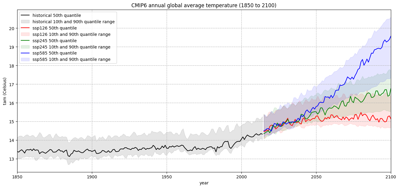
The visualization of the CMIP6 annual global average temperature (1850 to 2100) above shows that the global average temperature was more or less stable in the pre-industrial phase, but steadily increases since the 1990s. It shows further that, depending on the SSP scenario, the course and increase of the global annual temperature differs. While for the best case SSP1-2.6 scenario, the global annual temperature could stabilize around 15 degC, in the worst case SSP5-8.5 scenario, the global annual temperature could increase to above 20 degC.

---

Key Messages to Take Home 📌

• When calculating an ensemble of models, it is best practice to use as many as possible for a more reliable output.

• Before using the ensemble of models, preparation steps include spatial and temporal aggregation of data and possible conversion of units of measure.

• To merge datasets from different models and experiments, additional data dimensions must be created specifying the model and experiment of each dataset.

• Using quantiles instead of ploting all values eases data visualization.

---

This project is licensed under APACHE License 2.0. | View on GitHub