

Analysis of the Earth’s Radiation Budget using the CERES product#
This notebook-tutorial provides an introduction to the use of the Cloud and Earth’s Radiant Energy System (CERES) Energy Balanced and Filled (EBAF) Earth’s Radiation Budget (ERB) data record for climate studies.
The notebook comprises the following sections:
Table of content#
Introduction
Search, download and view data
Climatology of the Earth’s Radiation Budget
3.1. Climatology of the top-of-atmosphere incoming solar radiation
3.2. Climatology of the top-of-atmosphere reflected solar flux
3.3. Climatology of the top-of-atmosphere outgoing longwave radiation
3.4. Climatology of the top-of-atmosphere net Earth’s radiation budget
Time series and trend analysis of the Earth’s Radiaton Budget
4.1. Time series and trend analysis of the top-of-atmosphere incoming solar radiation
4.2. Time series and trend analysis of the top-of-atmosphere reflected solar flux
4.3. Time series and trend analysis of the top-of-atmosphere outgoing longwave radiation
4.4. Time series and trend analysis of the top-of-atmosphere net Earth’s radiation budget
Conclusion
1. Introduction#
You will find further information about the dataset as well as the data in the Climate Data Store catalogue entry Earth’s Radiation Budget, sections “Overview”, “Download data” and “Documentation”:
2. Search, download and view data#
Before we begin, we must prepare our environment. This includes installing the Application Programming Interface (API) of the CDS, and importing the various python libraries that we will need.
How to access the notebooks#
This tutorial is in the form of a Jupyter notebook, written in Python 3.9.4. You will not need to install any software for the training as there are a number of free cloud-based services to create, edit, run and export Jupyter notebooks such as this. Here are some suggestions (simply click on one of the links below to run the notebook):
| Run the tutorial via free cloud platforms: |
 |
 |
 |
|---|
The cdsapi is used to download the data. This package is not included by default on most cloud platforms yet. You can use pip to install it:
!pip install cdsapi
Import libraries#
To run this notebook in your own environment, we advise you to install Anaconda, which contains most of the libraries you will need. You will also need to install the CDS API (!pip install cdsapi) for downloading data programatically from the CDS. It is also recommended to use Python 3.9.4 for the purpose of reproducibility and compatibility, with respect to the latest updates of the different libraries.
The data have been stored in files written in NetCDF format. To best handle these, we will import the library Xarray which is specifically designed for manipulating multidimensional arrays in the field of geosciences. The libraries Matplotlib and Cartopy will also be imported for plotting and visualising the analysed data. We will also import the libraries zipfile to work with zip-archives, OS to use OS-functions and pattern expansion, and urllib3 for disabling warnings for data download via CDS API.
# Libraries to work with zip-archives, OS functions and pattern expansion
import zipfile
import os

# Disable warnings for data download via API
import urllib3
urllib3.disable_warnings()

# CDS API library
import cdsapi

# Libraries for working with multidimensional arrays
import xarray as xr
import numpy as np
import pandas as pd
# Import a sublibrary method for the seasonal decomposition of the time series
from statsmodels.tsa.seasonal import seasonal_decompose

# Libraries for plotting and visualising the data
import matplotlib.pyplot as plt
import cartopy.crs as ccrs
from cartopy.mpl.ticker import (LongitudeFormatter, LatitudeFormatter)
Download Data Using CDS API#
Set up CDS API credentials#
We will request data from the Climate Data Store (CDS): https://cds.climate.copernicus.eu/cdsapp#!/home. If you do not have an account yet, please click on “login/register” at the right top and select “Create new account”. Once the registration process is finished, you will be able to login to the CDS and have a look at your favourite data.
We will request data from the CDS programmatically with the help of the CDS API.
First, we need to manually set the CDS API credentials.
To do so, we need to define two variables: URL and KEY.
To obtain these, first login to the CDS, then visit https://cds.climate.copernicus.eu/api-how-to and copy the string of characters listed after “key:”. Replace the ######### below with this string.
URL = 'https://cds.climate.copernicus.eu/api/v2'
KEY = '######################################'
Here we specify a data directory in which we will download our data and all output files that we will generate:
# Data directory for downloading the data
DATADIR = './'
# Filename for the zip file downloaded from the CDS
download_zip_file = os.path.join(DATADIR, 'ceres-erb-monthly.zip')
# Filename for the netCDF file which contain the merged contents of the monthly files.
merged_netcdf_file = os.path.join(DATADIR, 'ceres-erb-monthly.nc')
Search for data#
To search for data, visit the CDS website: https://cds.climate.copernicus.eu/cdsapp#!/home. Here you can search for CERES EBAF data using the search bar. The data we need for this use case is the Earth’s radiation budget from 1979 to present derived from satellite observations. This catalogue entry provides data from various sources: NASA CERES EBAF, NOAA/NCEI HIRS OLR, ESA Cloud-CCI, EUMETSAT’s CM SAF CLARA-A3, C3S CCI and C3S RMIB TSI.
After selecting the correct catalogue entry, we will specify the product family, the origin, the sensor on satellite (for CCI product family only), the type of variable, the type of climate data record, the time aggregation, the temporal and geographical coverage we are interested in. These can all be selected in the “Download data” tab. In this tab a form appears in which we will select the following parameters to download:
Product family:
CERES EBAF (Clouds and the Earth's Radiant Energy System (CERES) Energy Balanced And Filled (EBAF))Origin:
NASA (National Aeronautics and Space Administration)Variable:
all(useSelect allbutton)Climate data record type:
TCDR (Thematic Climate Data Record)Time aggregation:
MonthlyYear:
all(useSelect allbutton)Month:
all(useSelect allbutton)Geographical area:
Whole available regionFormat:
Compressed zip file (.zip)
If you have not already done so, you will need to accept the “terms & conditions” of the data before you can download it.
At the end of the download form, select “Show API request”. This will reveal a block of code, which you can simply copy and paste into a cell of your Jupyter Notebook (see cell below) …
Download data#
… Having copied the API request into the cell below, running this will retrieve and download the data you requested into your local directory. However, before you run the cell below, the terms and conditions of this particular dataset need to have been accepted in the CDS. The option to view and accept these conditions is given at the end of the download form, just above the “Show API request” option.
c = cdsapi.Client()
c.retrieve(
    'satellite-earth-radiation-budget',
    {
        'product_family': 'ceres_ebaf',
        'origin': 'nasa',
        'variable': ['incoming_shortwave_radiation',
                     'outgoing_longwave_radiation',
                     'outgoing_shortwave_radiation',
                    ],
        'cdr_type': 'tcdr',
        'time_aggregation': 'monthly',
        'year': ['%04d' % (year) for year in range(2000, 2023)],
        'month': ['%02d' % (month) for month in range(1, 13)],
        'format': 'zip',
    },
    download_zip_file
)
2023-12-08 10:12:41,751 INFO Welcome to the CDS
2023-12-08 10:12:41,753 INFO Sending request to https://cds.climate.copernicus.eu/api/v2/resources/satellite-earth-radiation-budget
2023-12-08 10:12:41,927 INFO Request is completed
2023-12-08 10:12:41,928 INFO Downloading https://download-0020.copernicus-climate.eu/cache-compute-0020/cache/data8/dataset-satellite-earth-radiation-budget-fc6eaaee-0bbb-4e03-99f1-9e43f857a439.zip to ./ceres-erb-monthly.zip (53.3M)
2023-12-08 10:12:52,562 INFO Download rate 5M/s
Result(content_length=55937978,content_type=application/zip,location=https://download-0020.copernicus-climate.eu/cache-compute-0020/cache/data8/dataset-satellite-earth-radiation-budget-fc6eaaee-0bbb-4e03-99f1-9e43f857a439.zip)
Inspect data#
The data have been downloaded. We can now unzip the archive and merge all files into one NetCDF file to inspect them. NetCDF is a commonly used format for array-oriented scientifc data. To read and process these data, we will make use of the Xarray library. Xarray is an open source project and Python package that makes working with labelled multi-dimensional arrays simple and efficient. We will read the data from our NetCDF file into an Xarray Dataset.
# Unzip the data. The dataset is splitted in monthly files.
with zipfile.ZipFile(download_zip_file, 'r') as zip_ref:
    filelist = [os.path.join(DATADIR, f) for f in zip_ref.namelist()]
    zip_ref.extractall(DATADIR)
# Ensure the filelist is in the correct order
filelist = sorted(filelist)

# Merge all unpacked files into one.
ds = xr.open_mfdataset(filelist)
ds.to_netcdf(merged_netcdf_file)

# Recursively delete unpacked data
for f in filelist:
    os.remove(f)

# Read data
ds_ceres = xr.open_dataset(merged_netcdf_file, decode_times=True, mask_and_scale=True)
Now we can query our newly created Xarray dataset…
ds_ceres
<xarray.Dataset>
Dimensions:         (lat: 180, lon: 360, time: 274)
Coordinates:
  * time            (time) datetime64[ns] 2000-03-15 2000-04-15 ... 2022-12-15
  * lat             (lat) float32 -89.5 -88.5 -87.5 -86.5 ... 87.5 88.5 89.5
  * lon             (lon) float32 0.5 1.5 2.5 3.5 ... 356.5 357.5 358.5 359.5
Data variables:
    solar_mon       (time, lat, lon) float32 ...
    toa_lw_all_mon  (time, lat, lon) float32 ...
    toa_sw_all_mon  (time, lat, lon) float32 ...
Attributes:
    title:                           CERES EBAF (Energy Balanced and Filled) ...
    institution:                     NASA/LaRC (Langley Research Center) Hamp...
    Conventions:                     CF-1.4
    comment:                         Climatology from 07/2005 to 06/2015
    version:                         Edition 4.2; Release Date December 9, 2022
    DOI:                             10.5067/TERRA-AQUA-NOAA20/CERES/EBAF-TOA...
    Fill_Value:                      Fill Value is -999.0
    DODS_EXTRA.Unlimited_Dimension:  time
history: 2023-03-05 19:21:10 GMT Hyrax-1.16.2 htt...- lat: 180
- lon: 360
- time: 274
- time(time)datetime64[ns]2000-03-15 ... 2022-12-15
- long_name :
- Time
- delta_t :
- 0000-00-01 00:00:00
array(['2000-03-15T00:00:00.000000000', '2000-04-15T00:00:00.000000000', '2000-05-15T00:00:00.000000000', ..., '2022-10-15T00:00:00.000000000', '2022-11-15T00:00:00.000000000', '2022-12-15T00:00:00.000000000'], dtype='datetime64[ns]') - lat(lat)float32-89.5 -88.5 -87.5 ... 88.5 89.5
- long_name :
- Latitude
- standard_name :
- latitude
- units :
- degrees_north
- valid_range :
- [-90. 90.]
array([-89.5, -88.5, -87.5, -86.5, -85.5, -84.5, -83.5, -82.5, -81.5, -80.5, -79.5, -78.5, -77.5, -76.5, -75.5, -74.5, -73.5, -72.5, -71.5, -70.5, -69.5, -68.5, -67.5, -66.5, -65.5, -64.5, -63.5, -62.5, -61.5, -60.5, -59.5, -58.5, -57.5, -56.5, -55.5, -54.5, -53.5, -52.5, -51.5, -50.5, -49.5, -48.5, -47.5, -46.5, -45.5, -44.5, -43.5, -42.5, -41.5, -40.5, -39.5, -38.5, -37.5, -36.5, -35.5, -34.5, -33.5, -32.5, -31.5, -30.5, -29.5, -28.5, -27.5, -26.5, -25.5, -24.5, -23.5, -22.5, -21.5, -20.5, -19.5, -18.5, -17.5, -16.5, -15.5, -14.5, -13.5, -12.5, -11.5, -10.5, -9.5, -8.5, -7.5, -6.5, -5.5, -4.5, -3.5, -2.5, -1.5, -0.5, 0.5, 1.5, 2.5, 3.5, 4.5, 5.5, 6.5, 7.5, 8.5, 9.5, 10.5, 11.5, 12.5, 13.5, 14.5, 15.5, 16.5, 17.5, 18.5, 19.5, 20.5, 21.5, 22.5, 23.5, 24.5, 25.5, 26.5, 27.5, 28.5, 29.5, 30.5, 31.5, 32.5, 33.5, 34.5, 35.5, 36.5, 37.5, 38.5, 39.5, 40.5, 41.5, 42.5, 43.5, 44.5, 45.5, 46.5, 47.5, 48.5, 49.5, 50.5, 51.5, 52.5, 53.5, 54.5, 55.5, 56.5, 57.5, 58.5, 59.5, 60.5, 61.5, 62.5, 63.5, 64.5, 65.5, 66.5, 67.5, 68.5, 69.5, 70.5, 71.5, 72.5, 73.5, 74.5, 75.5, 76.5, 77.5, 78.5, 79.5, 80.5, 81.5, 82.5, 83.5, 84.5, 85.5, 86.5, 87.5, 88.5, 89.5], dtype=float32) - lon(lon)float320.5 1.5 2.5 ... 357.5 358.5 359.5
- long_name :
- Longitude
- standard_name :
- longitude
- units :
- degrees_east
- valid_range :
- [ 0. 360.]
array([ 0.5, 1.5, 2.5, ..., 357.5, 358.5, 359.5], dtype=float32)
- solar_mon(time, lat, lon)float32...
- long_name :
- Incoming Solar Flux, Monthly Means
- standard_name :
- Incoming Solar Flux
- CF_name :
- toa_incoming_shortwave_flux
- comment :
- none
- units :
- W m-2
- valid_min :
- 0.0
- valid_max :
- 800.0
[17755200 values with dtype=float32]
- toa_lw_all_mon(time, lat, lon)float32...
- long_name :
- Top of The Atmosphere Longwave Flux, All-Sky conditions, Monthly Means
- standard_name :
- TOA Longwave Flux - All-Sky
- CF_name :
- toa_outgoing_longwave_flux
- comment :
- none
- units :
- W m-2
- valid_min :
- 0.0
- valid_max :
- 400.0
[17755200 values with dtype=float32]
- toa_sw_all_mon(time, lat, lon)float32...
- long_name :
- Top of The Atmosphere Shortwave Flux, All-Sky conditions, Monthly Means
- standard_name :
- TOA Shortwave Flux - All-Sky
- CF_name :
- toa_outgoing_shortwave_flux
- comment :
- none
- units :
- W m-2
- valid_min :
- 0.0
- valid_max :
- 600.0
[17755200 values with dtype=float32]
- title :
- CERES EBAF (Energy Balanced and Filled) TOA Fluxes. Monthly Averages and 07/2005 to 06/2015 Climatology.
- institution :
- NASA/LaRC (Langley Research Center) Hampton, Va
- Conventions :
- CF-1.4
- comment :
- Climatology from 07/2005 to 06/2015
- version :
- Edition 4.2; Release Date December 9, 2022
- DOI :
- 10.5067/TERRA-AQUA-NOAA20/CERES/EBAF-TOA_L3B004.2
- Fill_Value :
- Fill Value is -999.0
- DODS_EXTRA.Unlimited_Dimension :
- time
- history :
- 2023-03-05 19:21:10 GMT Hyrax-1.16.2 https://opendap.larc.nasa.gov/opendap/CERES/EBAF/TOA_Edition4.2/CERES_EBAF-TOA_Edition4.2_200003-202211.nc.nc?solar_mon%5B0%5D%5B0:179%5D%5B0:359%5D
We see that the dataset has three variables solar_mon, toa_lw_all_mon and toa_sw_all_mon which stand for the incoming solar flux, the top of atmosphere (TOA) longwave (LW) and shortwave (SW) fluxes respectively, as well as three dimension coordinates of lon, lat and time.
While an Xarray dataset may contain multiple variables, an Xarray data array holds a single multi-dimensional variable and its coordinates. To make the processing of the solar_mon, toa_lw_all_mon and toa_sw_all_mon data easier, we convert them into three distinct Xarray data arrays. We can also define a new data array da_toa_erb that corresponds to the TOA net Earth’s radative budget and is defined as the difference between the incoming solar flux and the sum of the outgoing (LW, SW) fluxes at the top the atmosphere.
# Outgoing longwave radiation data array
da_toa_lw = ds_ceres['toa_lw_all_mon']

# Incoming shortwave radiation data array
da_solar = ds_ceres['solar_mon']

# Outgoing shortwave radiation data array
da_toa_sw = ds_ceres['toa_sw_all_mon']

# Creation of the net radiative flux data array
da_toa_erb = da_solar - da_toa_sw - da_toa_lw
# Name of the data array
da_toa_erb.name = 'toa_erb_all_mon'
# Add some attributes to the new data array
da_toa_erb.attrs = {
    'long_name': "Top of The Atmosphere Net Earth's Radiative Flux",
    'standard_name': "TOA Net Flux",'CF_name': "toa_net_radiative_flux",
    'comment': "none",
    'units': "W.m$^{-2}$",
                   }
Let us view these data, e.g. the toa_erb_all_mon data from our newly created da_toa_erb data array:
da_toa_erb
<xarray.DataArray 'toa_erb_all_mon' (time: 274, lat: 180, lon: 360)>
array([[[-126.02    , -126.02    , -126.02    , ..., -126.02    ,
         -126.02    , -126.02    ],
        [-124.909996, -124.909996, -124.909996, ..., -124.909996,
         -124.909996, -124.909996],
        [-124.34999 , -124.34999 , -124.34999 , ..., -124.34999 ,
         -124.34999 , -124.34999 ],
        ...,
        [-168.57    , -168.57    , -168.57    , ..., -168.57    ,
         -168.57    , -168.57    ],
        [-168.98    , -168.98    , -168.98    , ..., -168.98    ,
         -168.98    , -168.98    ],
        [-172.40001 , -172.40001 , -172.40001 , ..., -172.40001 ,
         -172.40001 , -172.40001 ]],

       [[-124.162   , -124.162   , -124.162   , ..., -124.162   ,
         -124.162   , -124.162   ],
        [-124.28    , -124.28    , -124.28    , ..., -124.28    ,
         -124.28    , -124.28    ],
        [-125.229   , -125.229   , -125.229   , ..., -125.229   ,
         -125.229   , -125.229   ],
...
        [-177.049   , -177.049   , -177.049   , ..., -177.049   ,
         -177.049   , -177.049   ],
        [-175.149   , -175.149   , -175.149   , ..., -175.149   ,
         -175.149   , -175.149   ],
        [-174.549   , -174.549   , -174.549   , ..., -174.549   ,
         -174.549   , -174.549   ]],

       [[ -19.59999 ,  -19.59999 ,  -19.59999 , ...,  -19.59999 ,
          -19.59999 ,  -19.59999 ],
        [ -16.699982,  -16.699982,  -16.699982, ...,  -16.699982,
          -16.699982,  -16.699982],
        [ -12.900009,  -12.900009,  -12.900009, ...,  -12.900009,
          -12.900009,  -12.900009],
        ...,
        [-172.546   , -172.546   , -172.546   , ..., -172.546   ,
         -172.546   , -172.546   ],
        [-171.746   , -171.746   , -171.746   , ..., -171.746   ,
         -171.746   , -171.746   ],
        [-171.147   , -171.147   , -171.147   , ..., -171.147   ,
         -171.147   , -171.147   ]]], dtype=float32)
Coordinates:
  * time     (time) datetime64[ns] 2000-03-15 2000-04-15 ... 2022-12-15
  * lat      (lat) float32 -89.5 -88.5 -87.5 -86.5 -85.5 ... 86.5 87.5 88.5 89.5
  * lon      (lon) float32 0.5 1.5 2.5 3.5 4.5 ... 355.5 356.5 357.5 358.5 359.5
Attributes:
    long_name:      Top of The Atmosphere Net Earth's Radiative Flux
    standard_name:  TOA Net Flux
    CF_name:        toa_net_radiative_flux
    comment:        none
units: W.m$^{-2}$- time: 274
- lat: 180
- lon: 360
- -126.0 -126.0 -126.0 -126.0 -126.0 ... -171.1 -171.1 -171.1 -171.1
array([[[-126.02 , -126.02 , -126.02 , ..., -126.02 , -126.02 , -126.02 ], [-124.909996, -124.909996, -124.909996, ..., -124.909996, -124.909996, -124.909996], [-124.34999 , -124.34999 , -124.34999 , ..., -124.34999 , -124.34999 , -124.34999 ], ..., [-168.57 , -168.57 , -168.57 , ..., -168.57 , -168.57 , -168.57 ], [-168.98 , -168.98 , -168.98 , ..., -168.98 , -168.98 , -168.98 ], [-172.40001 , -172.40001 , -172.40001 , ..., -172.40001 , -172.40001 , -172.40001 ]], [[-124.162 , -124.162 , -124.162 , ..., -124.162 , -124.162 , -124.162 ], [-124.28 , -124.28 , -124.28 , ..., -124.28 , -124.28 , -124.28 ], [-125.229 , -125.229 , -125.229 , ..., -125.229 , -125.229 , -125.229 ], ... [-177.049 , -177.049 , -177.049 , ..., -177.049 , -177.049 , -177.049 ], [-175.149 , -175.149 , -175.149 , ..., -175.149 , -175.149 , -175.149 ], [-174.549 , -174.549 , -174.549 , ..., -174.549 , -174.549 , -174.549 ]], [[ -19.59999 , -19.59999 , -19.59999 , ..., -19.59999 , -19.59999 , -19.59999 ], [ -16.699982, -16.699982, -16.699982, ..., -16.699982, -16.699982, -16.699982], [ -12.900009, -12.900009, -12.900009, ..., -12.900009, -12.900009, -12.900009], ..., [-172.546 , -172.546 , -172.546 , ..., -172.546 , -172.546 , -172.546 ], [-171.746 , -171.746 , -171.746 , ..., -171.746 , -171.746 , -171.746 ], [-171.147 , -171.147 , -171.147 , ..., -171.147 , -171.147 , -171.147 ]]], dtype=float32) - time(time)datetime64[ns]2000-03-15 ... 2022-12-15
- long_name :
- Time
- delta_t :
- 0000-00-01 00:00:00
array(['2000-03-15T00:00:00.000000000', '2000-04-15T00:00:00.000000000', '2000-05-15T00:00:00.000000000', ..., '2022-10-15T00:00:00.000000000', '2022-11-15T00:00:00.000000000', '2022-12-15T00:00:00.000000000'], dtype='datetime64[ns]') - lat(lat)float32-89.5 -88.5 -87.5 ... 88.5 89.5
- long_name :
- Latitude
- standard_name :
- latitude
- units :
- degrees_north
- valid_range :
- [-90. 90.]
array([-89.5, -88.5, -87.5, -86.5, -85.5, -84.5, -83.5, -82.5, -81.5, -80.5, -79.5, -78.5, -77.5, -76.5, -75.5, -74.5, -73.5, -72.5, -71.5, -70.5, -69.5, -68.5, -67.5, -66.5, -65.5, -64.5, -63.5, -62.5, -61.5, -60.5, -59.5, -58.5, -57.5, -56.5, -55.5, -54.5, -53.5, -52.5, -51.5, -50.5, -49.5, -48.5, -47.5, -46.5, -45.5, -44.5, -43.5, -42.5, -41.5, -40.5, -39.5, -38.5, -37.5, -36.5, -35.5, -34.5, -33.5, -32.5, -31.5, -30.5, -29.5, -28.5, -27.5, -26.5, -25.5, -24.5, -23.5, -22.5, -21.5, -20.5, -19.5, -18.5, -17.5, -16.5, -15.5, -14.5, -13.5, -12.5, -11.5, -10.5, -9.5, -8.5, -7.5, -6.5, -5.5, -4.5, -3.5, -2.5, -1.5, -0.5, 0.5, 1.5, 2.5, 3.5, 4.5, 5.5, 6.5, 7.5, 8.5, 9.5, 10.5, 11.5, 12.5, 13.5, 14.5, 15.5, 16.5, 17.5, 18.5, 19.5, 20.5, 21.5, 22.5, 23.5, 24.5, 25.5, 26.5, 27.5, 28.5, 29.5, 30.5, 31.5, 32.5, 33.5, 34.5, 35.5, 36.5, 37.5, 38.5, 39.5, 40.5, 41.5, 42.5, 43.5, 44.5, 45.5, 46.5, 47.5, 48.5, 49.5, 50.5, 51.5, 52.5, 53.5, 54.5, 55.5, 56.5, 57.5, 58.5, 59.5, 60.5, 61.5, 62.5, 63.5, 64.5, 65.5, 66.5, 67.5, 68.5, 69.5, 70.5, 71.5, 72.5, 73.5, 74.5, 75.5, 76.5, 77.5, 78.5, 79.5, 80.5, 81.5, 82.5, 83.5, 84.5, 85.5, 86.5, 87.5, 88.5, 89.5], dtype=float32) - lon(lon)float320.5 1.5 2.5 ... 357.5 358.5 359.5
- long_name :
- Longitude
- standard_name :
- longitude
- units :
- degrees_east
- valid_range :
- [ 0. 360.]
array([ 0.5, 1.5, 2.5, ..., 357.5, 358.5, 359.5], dtype=float32)
- long_name :
- Top of The Atmosphere Net Earth's Radiative Flux
- standard_name :
- TOA Net Flux
- CF_name :
- toa_net_radiative_flux
- comment :
- none
- units :
- W.m$^{-2}$
Plot data#
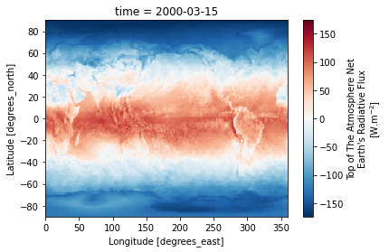
We can visualize one time step to figure out what the data look like. Xarray offers built-in matplotlib functions that allow you to plot a DataArray. With the function plot(), you can easily plot e.g. the first time step of the loaded array.
da_toa_erb[0, :, :].plot()
<matplotlib.collections.QuadMesh at 0x7f44763316a0>
An alternative to the built-in Xarray plotting functions is to make use of a combination of the plotting libraries matplotlib and Cartopy. One of Cartopy’s key features is its ability to transform array data into different geographic projections. In combination with matplotlib, it is a very powerful way to create high-quality visualisations and animations. In later plots, we will make use of these libraries to produce more customised visualisations.
3. Climatology of the Earth’s Radiation Budget#
3.1. Climatology of the top-of-atmosphere incoming solar radiation#
Time averaged global climatological distribution of TIS#
To calculate the mean climatology of the top of the atmosphere incoming solar radiation for the time period January 2001 to December 2021, we have to select the specific time range using the Xarray method sel() that indexes the data and dimensions by the appropriate indexers. We can then use the method mean() to calculate the mean along the time dimension.
# Select the TOA incoming solar radiation data for the whole time period
solar = da_solar.sel(time=slice('2001-01-01', '2021-12-31'))

# Calculate the mean along the time dimension
solar_mean = solar.mean(dim='time')
We can now visualize the time averaged global climatological distribution of the incoming solar radiation for the period January 2001 - December 2021. This time, we will make use of a combination of the plotting libraries Matplotlib and Cartopy to create a more customised figure.
# Create the figure panel and the map using the Cartopy PlateCarree projection
fig1, ax1 = plt.subplots(1, 1, figsize=(16, 8), subplot_kw={'projection': ccrs.PlateCarree()})

# Plot the data
im = plt.pcolormesh(solar_mean.lon, solar_mean.lat, solar_mean, cmap='YlOrRd')

# Set the figure title, add lat/lon grid and coastlines
ax1.set_title(
    '$\\bf{Climatology\ of\ TIS\ from\ CERES\ EBAF\ (January\ 2001\ -\ December\ 2021)}$',
    fontsize=20,
    pad=20)
# Add coastlines
ax1.coastlines(color='black')
# Define gridlines and ticks
ax1.set_xticks(np.arange(-180, 181, 60), crs=ccrs.PlateCarree())
ax1.set_yticks(np.arange(-90, 91, 30), crs=ccrs.PlateCarree())
lon_formatter = LongitudeFormatter()
lat_formatter = LatitudeFormatter()
ax1.xaxis.set_major_formatter(lon_formatter)
ax1.yaxis.set_major_formatter(lat_formatter)
# Gridlines
gl = ax1.gridlines(linewidth=1, color='gray', alpha=0.5, linestyle='--')

# Specify the colorbar
cbar = plt.colorbar(im, fraction=0.025, pad=0.05, extend='both')
cbar.set_label('W.m$^{-2}$')

# Save the figure
fig1.savefig(f'{DATADIR}ceres_solar_climatology.png')
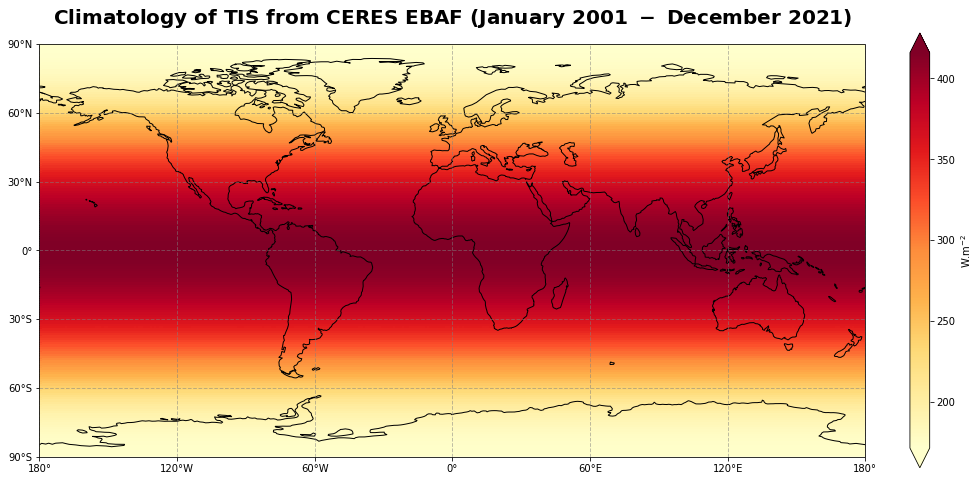
Figure 1 shows the regular latitude dependent climatological distribution of the incoming solar radiation at the top of the atmosphere, with values decreasing from the tropics to the high latitudes.
Time averaged seasonal climatological distribution of TIS#
The TOA incoming solar radiation data can also be splitted according to the seasons by using the groupby() method, with 'time.season' as an argument, and then averaged over the years.
Seasons are defined as follows, using the Northern Hemisphere (NH) as reference:
NH spring: March, April, May
NH summer: June, July, August
NH autumn: September, October, November
NH winter: December, January, February
# Split data array solar by season
solar_seasonal_climatology = solar.groupby('time.season').mean('time')
solar_seasonal_climatology
<xarray.DataArray 'solar_mon' (season: 4, lat: 180, lon: 360)>
array([[[450.3857  , 450.3857  , 450.3857  , ..., 450.3857  ,
         450.3857  , 450.3857  ],
        [450.2461  , 450.2461  , 450.2461  , ..., 450.2461  ,
         450.2461  , 450.2461  ],
        [449.9793  , 449.9793  , 449.9793  , ..., 449.9793  ,
         449.9793  , 449.9793  ],
        ...,
        [  0.      ,   0.      ,   0.      , ...,   0.      ,
           0.      ,   0.      ],
        [  0.      ,   0.      ,   0.      , ...,   0.      ,
           0.      ,   0.      ],
        [  0.      ,   0.      ,   0.      , ...,   0.      ,
           0.      ,   0.      ]],

       [[  0.      ,   0.      ,   0.      , ...,   0.      ,
           0.      ,   0.      ],
        [  0.      ,   0.      ,   0.      , ...,   0.      ,
           0.      ,   0.      ],
        [  0.      ,   0.      ,   0.      , ...,   0.      ,
           0.      ,   0.      ],
...
        [229.18077 , 229.18077 , 229.18077 , ..., 229.18077 ,
         229.18077 , 229.18077 ],
        [228.66728 , 228.66728 , 228.66728 , ..., 228.66728 ,
         228.66728 , 228.66728 ],
        [228.41019 , 228.41019 , 228.41019 , ..., 228.41019 ,
         228.41019 , 228.41019 ]],

       [[221.11821 , 221.11821 , 221.11821 , ..., 221.11821 ,
         221.11821 , 221.11821 ],
        [221.38689 , 221.38689 , 221.38689 , ..., 221.38689 ,
         221.38689 , 221.38689 ],
        [221.92633 , 221.92633 , 221.92633 , ..., 221.92633 ,
         221.92633 , 221.92633 ],
        ...,
        [ 25.165077,  25.165077,  25.165077, ...,  25.165077,
          25.165077,  25.165077],
        [ 24.507938,  24.507938,  24.507938, ...,  24.507938,
          24.507938,  24.507938],
        [ 24.182222,  24.182222,  24.182222, ...,  24.182222,
          24.182222,  24.182222]]], dtype=float32)
Coordinates:
  * lat      (lat) float32 -89.5 -88.5 -87.5 -86.5 -85.5 ... 86.5 87.5 88.5 89.5
  * lon      (lon) float32 0.5 1.5 2.5 3.5 4.5 ... 355.5 356.5 357.5 358.5 359.5
* season (season) object 'DJF' 'JJA' 'MAM' 'SON'- season: 4
- lat: 180
- lon: 360
- 450.4 450.4 450.4 450.4 450.4 450.4 ... 24.18 24.18 24.18 24.18 24.18
array([[[450.3857 , 450.3857 , 450.3857 , ..., 450.3857 , 450.3857 , 450.3857 ], [450.2461 , 450.2461 , 450.2461 , ..., 450.2461 , 450.2461 , 450.2461 ], [449.9793 , 449.9793 , 449.9793 , ..., 449.9793 , 449.9793 , 449.9793 ], ..., [ 0. , 0. , 0. , ..., 0. , 0. , 0. ], [ 0. , 0. , 0. , ..., 0. , 0. , 0. ], [ 0. , 0. , 0. , ..., 0. , 0. , 0. ]], [[ 0. , 0. , 0. , ..., 0. , 0. , 0. ], [ 0. , 0. , 0. , ..., 0. , 0. , 0. ], [ 0. , 0. , 0. , ..., 0. , 0. , 0. ], ... [229.18077 , 229.18077 , 229.18077 , ..., 229.18077 , 229.18077 , 229.18077 ], [228.66728 , 228.66728 , 228.66728 , ..., 228.66728 , 228.66728 , 228.66728 ], [228.41019 , 228.41019 , 228.41019 , ..., 228.41019 , 228.41019 , 228.41019 ]], [[221.11821 , 221.11821 , 221.11821 , ..., 221.11821 , 221.11821 , 221.11821 ], [221.38689 , 221.38689 , 221.38689 , ..., 221.38689 , 221.38689 , 221.38689 ], [221.92633 , 221.92633 , 221.92633 , ..., 221.92633 , 221.92633 , 221.92633 ], ..., [ 25.165077, 25.165077, 25.165077, ..., 25.165077, 25.165077, 25.165077], [ 24.507938, 24.507938, 24.507938, ..., 24.507938, 24.507938, 24.507938], [ 24.182222, 24.182222, 24.182222, ..., 24.182222, 24.182222, 24.182222]]], dtype=float32) - lat(lat)float32-89.5 -88.5 -87.5 ... 88.5 89.5
- long_name :
- Latitude
- standard_name :
- latitude
- units :
- degrees_north
- valid_range :
- [-90. 90.]
array([-89.5, -88.5, -87.5, -86.5, -85.5, -84.5, -83.5, -82.5, -81.5, -80.5, -79.5, -78.5, -77.5, -76.5, -75.5, -74.5, -73.5, -72.5, -71.5, -70.5, -69.5, -68.5, -67.5, -66.5, -65.5, -64.5, -63.5, -62.5, -61.5, -60.5, -59.5, -58.5, -57.5, -56.5, -55.5, -54.5, -53.5, -52.5, -51.5, -50.5, -49.5, -48.5, -47.5, -46.5, -45.5, -44.5, -43.5, -42.5, -41.5, -40.5, -39.5, -38.5, -37.5, -36.5, -35.5, -34.5, -33.5, -32.5, -31.5, -30.5, -29.5, -28.5, -27.5, -26.5, -25.5, -24.5, -23.5, -22.5, -21.5, -20.5, -19.5, -18.5, -17.5, -16.5, -15.5, -14.5, -13.5, -12.5, -11.5, -10.5, -9.5, -8.5, -7.5, -6.5, -5.5, -4.5, -3.5, -2.5, -1.5, -0.5, 0.5, 1.5, 2.5, 3.5, 4.5, 5.5, 6.5, 7.5, 8.5, 9.5, 10.5, 11.5, 12.5, 13.5, 14.5, 15.5, 16.5, 17.5, 18.5, 19.5, 20.5, 21.5, 22.5, 23.5, 24.5, 25.5, 26.5, 27.5, 28.5, 29.5, 30.5, 31.5, 32.5, 33.5, 34.5, 35.5, 36.5, 37.5, 38.5, 39.5, 40.5, 41.5, 42.5, 43.5, 44.5, 45.5, 46.5, 47.5, 48.5, 49.5, 50.5, 51.5, 52.5, 53.5, 54.5, 55.5, 56.5, 57.5, 58.5, 59.5, 60.5, 61.5, 62.5, 63.5, 64.5, 65.5, 66.5, 67.5, 68.5, 69.5, 70.5, 71.5, 72.5, 73.5, 74.5, 75.5, 76.5, 77.5, 78.5, 79.5, 80.5, 81.5, 82.5, 83.5, 84.5, 85.5, 86.5, 87.5, 88.5, 89.5], dtype=float32) - lon(lon)float320.5 1.5 2.5 ... 357.5 358.5 359.5
- long_name :
- Longitude
- standard_name :
- longitude
- units :
- degrees_east
- valid_range :
- [ 0. 360.]
array([ 0.5, 1.5, 2.5, ..., 357.5, 358.5, 359.5], dtype=float32)
- season(season)object'DJF' 'JJA' 'MAM' 'SON'
array(['DJF', 'JJA', 'MAM', 'SON'], dtype=object)
The xarray solar_seasonal_climatology has four entries in the time dimension (one for each season). The climatology of the incident solar flux distribution can now be plotted for each season.
# Create a list of the seasons such as defined in the dataset solar_seasonal_climatology:
seasons = ['MAM', 'JJA', 'SON', 'DJF']

# We use the "subplots" to place multiple plots according to our needs.
# In this case, we want 4 plots in a 2x2 format.
# For this "nrows" = 2 and "ncols" = 2, the projection and size are defined as well
fig2, ax2 = plt.subplots(nrows=2,
                         ncols=2,
                         subplot_kw={'projection': ccrs.PlateCarree()},
                         figsize=(16,8))

# Define a dictionary of subtitles, each one corresponding to a season
subtitles = {'MAM': 'NH spring', 'JJA': 'NH summer', 'SON': 'NH autumn', 'DJF': 'NH winter'}

# Configure the axes and subplot titles
for i_season, c_season in enumerate(seasons):
    # convert i_season index into (row, col) index
    row = i_season // 2
    col = i_season % 2
    # Plot data (coordinates and data) and define colormap
    im = ax2[row][col].pcolormesh(solar_seasonal_climatology.lon,
                                  solar_seasonal_climatology.lat,
                                  solar_seasonal_climatology.sel(season=c_season),
                                  cmap='YlOrRd')
    # Set title and size
    ax2[row][col].set_title('Seasonal climatology of TIS - ' + subtitles[c_season], fontsize=16)
    # Add coastlines
    ax2[row][col].coastlines()
    # Define grid lines and ticks (e.g. from -180 to 180 in an interval of 60)
    ax2[row][col].set_xticks(np.arange(-180, 181, 60), crs=ccrs.PlateCarree())
    ax2[row][col].set_yticks(np.arange(-90, 91, 30), crs=ccrs.PlateCarree())
    lon_formatter = LongitudeFormatter()
    lat_formatter = LatitudeFormatter()
    ax2[row][col].xaxis.set_major_formatter(lon_formatter)
    ax2[row][col].yaxis.set_major_formatter(lat_formatter)
    # Gridline
    gl = ax2[row][col].gridlines(linewidth=1, color='gray', alpha=0.5, linestyle='--')

# Place the subplots
fig2.subplots_adjust(bottom=0.0, top=0.9, left=0.05, right=0.95, wspace=0.1, hspace=0.5)

# Define and place a colorbar at the bottom
cbar_ax = fig2.add_axes([0.2, -0.1, 0.6, 0.02])
cbar = fig2.colorbar(im, cax=cbar_ax, orientation='horizontal', extend='both')
cbar.set_label('W.m$^{-2}$', fontsize=16)

# Define an overall title
fig2.suptitle('$\\bf{Seasonal\ climatology\ of\ TIS\ from\ CERES\ EBAF\ (January\ 2001\ -\ December\ 2021)}$',
              fontsize=20)

# Save the figure
fig2.savefig(f'{DATADIR}ceres_solar_seasonal_climatology.png')
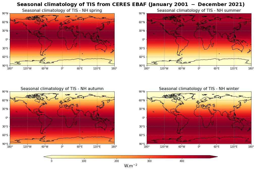
Figure 2 shows the seasonal mean climatology of the top of the atmosphere incoming solar radiation from spring to winter (top left to bottom right panels) derived from CERES EBAF.
Zonally averaged montly mean climatology of TIS#
We will now calculate the monthly mean climatology of the top-of-atmosphere incoming solar radiation over the time period January 2001 - December 2021 by first applying the groupby() method to group the data array by month and then calculating the average for each monthly group. The resulting data array is the monthly climatology for the top of atmosphere incident solar radiation based on reference January 2001 - December 2021.
solar_clim_month = solar.groupby('time.month').mean("time")
Let us view the zonal monthly climatology of the TOA incoming solar radiation. To do this, we will average across the longitude bands with the mean() method, align the time dimension coordinate with the x axis and the lat dimension coordinate along the y axis using the method transpose()…
solar_zonal_clim_month = solar_clim_month.mean(dim="lon").transpose()
solar_zonal_clim_month
<xarray.DataArray 'solar_mon' (lat: 180, month: 12)>
array([[495.919   , 305.7905  ,  58.86096 , ..., 212.30956 , 440.9857  ,
        549.4477  ],
       [495.75546 , 305.69235 ,  59.817547, ..., 212.24393 , 440.8527  ,
        549.279   ],
       [495.45468 , 305.51282 ,  61.73928 , ..., 212.10985 , 440.58533 ,
        548.948   ],
       ...,
       [  0.      ,   0.      ,  22.81825 , ...,   0.      ,   0.      ,
          0.      ],
       [  0.      ,   0.      ,  20.87273 , ...,   0.      ,   0.      ,
          0.      ],
       [  0.      ,   0.      ,  19.901903, ...,   0.      ,   0.      ,
          0.      ]], dtype=float32)
Coordinates:
  * lat      (lat) float32 -89.5 -88.5 -87.5 -86.5 -85.5 ... 86.5 87.5 88.5 89.5
* month (month) int64 1 2 3 4 5 6 7 8 9 10 11 12- lat: 180
- month: 12
- 495.9 305.8 58.86 0.0 0.0 0.0 0.0 ... 473.7 309.2 72.55 0.0 0.0 0.0
array([[495.919 , 305.7905 , 58.86096 , ..., 212.30956 , 440.9857 , 549.4477 ], [495.75546 , 305.69235 , 59.817547, ..., 212.24393 , 440.8527 , 549.279 ], [495.45468 , 305.51282 , 61.73928 , ..., 212.10985 , 440.58533 , 548.948 ], ..., [ 0. , 0. , 22.81825 , ..., 0. , 0. , 0. ], [ 0. , 0. , 20.87273 , ..., 0. , 0. , 0. ], [ 0. , 0. , 19.901903, ..., 0. , 0. , 0. ]], dtype=float32) - lat(lat)float32-89.5 -88.5 -87.5 ... 88.5 89.5
- long_name :
- Latitude
- standard_name :
- latitude
- units :
- degrees_north
- valid_range :
- [-90. 90.]
array([-89.5, -88.5, -87.5, -86.5, -85.5, -84.5, -83.5, -82.5, -81.5, -80.5, -79.5, -78.5, -77.5, -76.5, -75.5, -74.5, -73.5, -72.5, -71.5, -70.5, -69.5, -68.5, -67.5, -66.5, -65.5, -64.5, -63.5, -62.5, -61.5, -60.5, -59.5, -58.5, -57.5, -56.5, -55.5, -54.5, -53.5, -52.5, -51.5, -50.5, -49.5, -48.5, -47.5, -46.5, -45.5, -44.5, -43.5, -42.5, -41.5, -40.5, -39.5, -38.5, -37.5, -36.5, -35.5, -34.5, -33.5, -32.5, -31.5, -30.5, -29.5, -28.5, -27.5, -26.5, -25.5, -24.5, -23.5, -22.5, -21.5, -20.5, -19.5, -18.5, -17.5, -16.5, -15.5, -14.5, -13.5, -12.5, -11.5, -10.5, -9.5, -8.5, -7.5, -6.5, -5.5, -4.5, -3.5, -2.5, -1.5, -0.5, 0.5, 1.5, 2.5, 3.5, 4.5, 5.5, 6.5, 7.5, 8.5, 9.5, 10.5, 11.5, 12.5, 13.5, 14.5, 15.5, 16.5, 17.5, 18.5, 19.5, 20.5, 21.5, 22.5, 23.5, 24.5, 25.5, 26.5, 27.5, 28.5, 29.5, 30.5, 31.5, 32.5, 33.5, 34.5, 35.5, 36.5, 37.5, 38.5, 39.5, 40.5, 41.5, 42.5, 43.5, 44.5, 45.5, 46.5, 47.5, 48.5, 49.5, 50.5, 51.5, 52.5, 53.5, 54.5, 55.5, 56.5, 57.5, 58.5, 59.5, 60.5, 61.5, 62.5, 63.5, 64.5, 65.5, 66.5, 67.5, 68.5, 69.5, 70.5, 71.5, 72.5, 73.5, 74.5, 75.5, 76.5, 77.5, 78.5, 79.5, 80.5, 81.5, 82.5, 83.5, 84.5, 85.5, 86.5, 87.5, 88.5, 89.5], dtype=float32) - month(month)int641 2 3 4 5 6 7 8 9 10 11 12
array([ 1, 2, 3, 4, 5, 6, 7, 8, 9, 10, 11, 12])
Now we can plot our data. Before we do this however, we define the min, max and step of contours that we will use in a contour plot.
# Define contour parameters (min, max and step)
vdiv = 5
vmin = 0
vmax = 500
clevs = np.arange(vmin, vmax, vdiv)
# Define the figure and specify size
fig3, ax3 = plt.subplots(1, 1, figsize=(16, 8))

# Configure the axes and figure title
ax3.set_xlabel('Month')
ax3.set_ylabel('Latitude [ $^o$ ]')
ax3.set_title(
    '$\\bf{Zonally\ averaged\ monthly\ climatology\ of\ TIS\ (January\ 2001\ -\ December\ 2021)}$',
    fontsize=20,
    pad=20)

# As the months (12) are much less than the latitudes (180),
# we need to ensure the plot fits into the size of the figure.
ax3.set_aspect('auto')

# Plot the data as a contour plot
contour = ax3.contourf(solar_zonal_clim_month.month,
                       solar_zonal_clim_month.lat,
                       solar_zonal_clim_month,
                       levels=clevs,
                       cmap='YlOrRd',
                       extend='both')
ax3.set_xticks(np.arange(1, 13, 1))
ax3.set_yticks(np.arange(-90, 91, 30))

# Specify the colorbar
cbar = plt.colorbar(contour, fraction=0.025, pad=0.05)
cbar.set_label('W.m$^{-2}$')

# Save the figure
fig3.savefig(f'{DATADIR}ceres_solar_monthly_climatology.png')
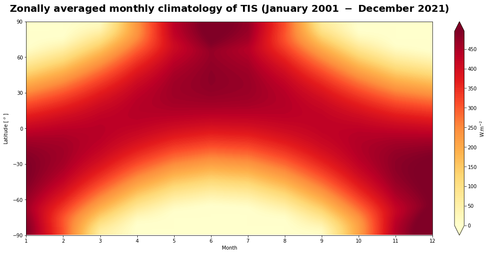
Figure 3 is a Hovmöller diagram that describes the annual variability of the incoming solar radiation at the top of the atmosphere with latitude over the time period January 2001 to December 2021. It is used in meteorology and for climate studies to show how a variable varies with latitude over time.
3.2. Climatology of the top-of-atmosphere reflected solar flux#
Time averaged global climatological distribution of TOA RSF#
To calculate the mean climatology of the top of the atmosphere reflected solar flux for the time period January 2001 to December 2021, we have to select the specific time range using the Xarray method sel() that indexes the data and dimensions by the appropriate indexers. We can then use the method mean() to calculate the mean along the time dimension.
# Select the TOA RSF data for the whole time period
toa_sw = da_toa_sw.sel(time=slice('2001-01-01', '2021-12-31'))

# Calculate the mean along the time dimension
toa_sw_mean = toa_sw.mean(dim='time')
We can now make use of a combination of the plotting libraries Matplotlib and Cartopy to create a customised figure and visualise the time averaged global climatological distribution of the TOA reflected solar flux for the period January 2001 - December 2021.
# Create the figure panel and the map using the Cartopy PlateCarree projection
fig4, ax4 = plt.subplots(1, 1, figsize=(16, 8), subplot_kw={'projection': ccrs.PlateCarree()})

# Plot the data
im = plt.pcolormesh(toa_sw_mean.lon, toa_sw_mean.lat, toa_sw_mean, cmap='YlOrRd')

# Set the figure title, add lat/lon grid and coastlines
ax4.set_title(
    '$\\bf{Climatology\ of\ TOA\ RSF\ from\ CERES\ EBAF\ (January\ 2001\ -\ December\ 2021)}$',
    fontsize=20,
    pad=20)
# Add coastlines
ax4.coastlines(color='black')
# Define gridlines and ticks
ax4.set_xticks(np.arange(-180, 181, 60), crs=ccrs.PlateCarree())
ax4.set_yticks(np.arange(-90, 91, 30), crs=ccrs.PlateCarree())
lon_formatter = LongitudeFormatter()
lat_formatter = LatitudeFormatter()
ax4.xaxis.set_major_formatter(lon_formatter)
ax4.yaxis.set_major_formatter(lat_formatter)
# Gridlines
gl = ax4.gridlines(linewidth=1, color='gray', alpha=0.5, linestyle='--')

# Specify the colorbar
cbar = plt.colorbar(im, fraction=0.025, pad=0.05, extend='both')
cbar.set_label('W.m$^{-2}$')

# Save the figure
fig4.savefig(f'{DATADIR}ceres_toa_sw_climatology.png')
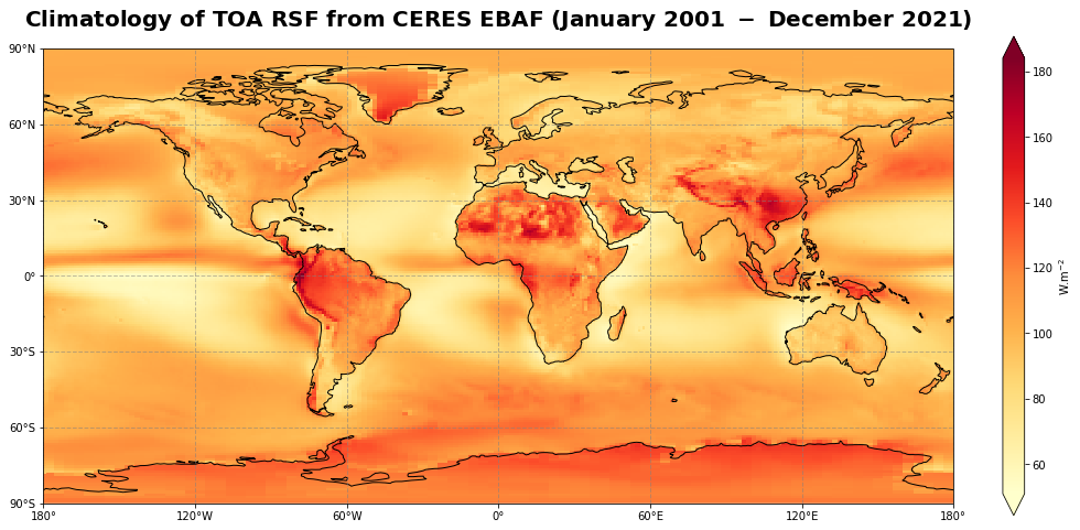
Figure 4 shows the global climatology of the top of the atmospohere reflected solar radiation for the time period of January 2001 - December 2021.
Time averaged seasonal climatological distribution of TOA RSF#
We now split the TOA RSF data according to the seasons by using the groupby() method, with 'time.season' as an argument, and then average them over the years.
# Split data array toa_sw by season
toa_sw_seasonal_climatology = toa_sw.groupby('time.season').mean('time')
# Create a list of the seasons such as defined in the dataset toa_sw_seasonal_climatology:
seasons = ['MAM', 'JJA', 'SON', 'DJF']

# We use the "subplots" to place multiple plots according to our needs.
# In this case, we want 4 plots in a 2x2 format.
# For this "nrows" = 2 and "ncols" = 2, the projection and size are defined as well
fig5, ax5 = plt.subplots(nrows=2,
                         ncols=2,
                         subplot_kw={'projection': ccrs.PlateCarree()},
                         figsize=(16,8))

# Define a dictionary of subtitles, each one corresponding to a season
subtitles = {'MAM': 'NH spring', 'JJA': 'NH summer', 'SON': 'NH autumn', 'DJF': 'NH winter'}

# Configure the axes and subplot titles
for i_season, c_season in enumerate(seasons):
    # convert i_season index into (row, col) index
    row = i_season // 2
    col = i_season % 2
    # Plot data (coordinates and data) and define colormap
    im = ax5[row][col].pcolormesh(toa_sw_seasonal_climatology.lon,
                                  toa_sw_seasonal_climatology.lat,
                                  toa_sw_seasonal_climatology.sel(season=c_season),
                                  cmap='YlOrRd')
    # Set title and size
    ax5[row][col].set_title('Seasonal climatology of TOA RSF - ' + subtitles[c_season], fontsize=16)
    # Add coastlines
    ax5[row][col].coastlines()
    # Define grid lines and ticks (e.g. from -180 to 180 in an interval of 60)
    ax5[row][col].set_xticks(np.arange(-180, 181, 60), crs=ccrs.PlateCarree())
    ax5[row][col].set_yticks(np.arange(-90, 91, 30), crs=ccrs.PlateCarree())
    lon_formatter = LongitudeFormatter()
    lat_formatter = LatitudeFormatter()
    ax5[row][col].xaxis.set_major_formatter(lon_formatter)
    ax5[row][col].yaxis.set_major_formatter(lat_formatter)
    # Gridline
    gl = ax5[row][col].gridlines(linewidth=1, color='gray', alpha=0.5, linestyle='--')

# Place the subplots
fig5.subplots_adjust(bottom=0.0, top=0.9, left=0.05, right=0.95, wspace=0.1, hspace=0.5)

# Define and place a colorbar at the bottom
cbar_ax = fig5.add_axes([0.2, -0.1, 0.6, 0.02])
cbar = fig5.colorbar(im, cax=cbar_ax, orientation='horizontal', extend='both')
cbar.set_label('W.m$^{-2}$', fontsize=16)

# Define an overall title
fig5.suptitle('$\\bf{Seasonal\ climatology\ of\ TOA\ RSF\ from\ CERES\ EBAF\ (January\ 2001\ -\ December\ 2021)}$',
              fontsize=20)

# Save the figure
fig5.savefig(f'{DATADIR}erb_toa_sw_seasonal_climatology.png')
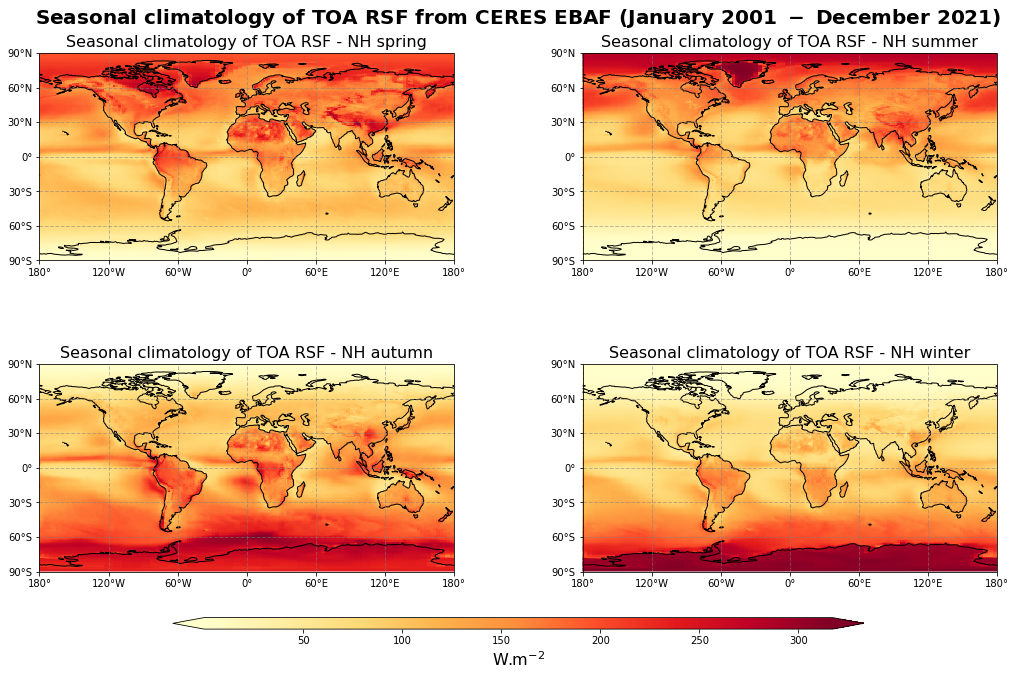
Figure 5 shows the seasonal mean climatology of the top of the atmosphere reflected solar flux from spring to winter (top left to bottom right panels) derived from CERES EBAF.
The influence of the albedo surfaces on the outgoing shorwave radiation observed in Figure 5 is confirmed by the seasonal climatology, with much higher values of TOA RSF over snow and ice in the summer Arctic and Antarctic regions.
Zonally averaged montly mean climatology of TOA RSF#
We will now calculate the monthly mean climatology of the outgoing shortwave radiation over the time period January 2001 - December 2021 by first applying the groupby() method to group the data array by month and then calculating the average for each monthly group. The resulting data array is the monthly climatology for the TOA reflected solar radiation based on reference January 2001 - December 2021.
toa_sw_clim_month = toa_sw.groupby('time.month').mean("time")
Before viewing the zonal monthly climatology of the TOA RSF, we must average across the longitude bands with the mean() method, align the time dimension coordinate with the x axis and the lat dimension coordinate along the y axis using the method transpose()…
toa_sw_zonal_clim_month = toa_sw_clim_month.mean(dim="lon").transpose()
Now we can plot our data. Before we do this however, we define the min, max and step of contours that we will use in a contour plot.
# Define contour parameters (min, max and step)
vdiv = 5
vmin = 0
vmax = 355
clevs = np.arange(vmin, vmax, vdiv)
# Define the figure and specify size
fig6, ax6 = plt.subplots(1, 1, figsize=(16, 8))

# Configure the axes and figure title
ax6.set_xlabel('Month')
ax6.set_ylabel('Latitude [ $^o$ ]')
ax6.set_title(
    '$\\bf{Zonally\ averaged\ monthly\ climatology\ of\ TOA\ RSF\ (January\ 2001\ -\ December\ 2021)}$',
    fontsize=20,
    pad=20)

# As the months (12) are much less than the latitudes (180),
# we need to ensure the plot fits into the size of the figure.
ax6.set_aspect('auto')

# Plot the data as a contour plot
contour = ax6.contourf(toa_sw_zonal_clim_month.month,
                       toa_sw_zonal_clim_month.lat,
                       toa_sw_zonal_clim_month,
                       levels=clevs,
                       cmap='YlOrRd',
                       extend='both')
ax6.set_xticks(np.arange(1, 13, 1))
ax6.set_yticks(np.arange(-90, 91, 30))

# Specify the colorbar
cbar = plt.colorbar(contour, fraction=0.025, pad=0.05)
cbar.set_label('W.m$^{-2}$')

# Save the figure
fig6.savefig(f'{DATADIR}ceres_toa_sw_monthly_climatology.png')
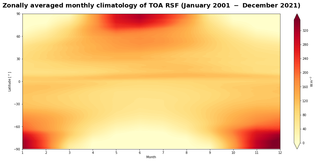
Figure 6 shows the seasonal variation of the top the atmosphere shortwave flux.
3.3. Climatology of the top-of-atmosphere outgoing longwave radiation#
Time averaged global climatological distribution of TOA OLR#
To calculate the mean climatology of the TOA outgoing longwave radiation for the period January 2001 to December 2021, we select the specific time range using the Xarray method sel() that indexes the data and dimensions by the appropriate indexers. We then use the method mean() to calculate the mean along the time dimension.
# Select the OLR data for the whole time period
toa_lw = da_toa_lw.sel(time=slice('2001-01-01', '2021-12-31'))

# Calculate the mean along the time dimension
toa_lw_mean = toa_lw.mean(dim='time')
We now make use of a combination of the plotting libraries Matplotlib and Cartopy to visualise the time averaged global climatological distribution of the TOA longwave radiation for the period January 2001 - December 2021.
# Create the figure panel and the map using the Cartopy PlateCarree projection
fig7, ax7 = plt.subplots(1, 1, figsize=(16, 8), subplot_kw={'projection': ccrs.PlateCarree()})

# Plot the data
im = plt.pcolormesh(toa_lw_mean.lon, toa_lw_mean.lat, toa_lw_mean, cmap='YlOrRd')

# Set the figure title, add lat/lon grid and coastlines
ax7.set_title(
    '$\\bf{Climatology\ of\ OLR\ from\ CERES\ EBAF\ (January\ 2001\ -\ December\ 2021)}$',
    fontsize=20,
    pad=20)
# Add coastlines
ax7.coastlines(color='black')
# Define gridlines and ticks
ax7.set_xticks(np.arange(-180, 181, 60), crs=ccrs.PlateCarree())
ax7.set_yticks(np.arange(-90, 91, 30), crs=ccrs.PlateCarree())
lon_formatter = LongitudeFormatter()
lat_formatter = LatitudeFormatter()
ax7.xaxis.set_major_formatter(lon_formatter)
ax7.yaxis.set_major_formatter(lat_formatter)
# Gridlines
gl = ax7.gridlines(linewidth=1, color='gray', alpha=0.5, linestyle='--')

# Specify the colorbar
cbar = plt.colorbar(im, fraction=0.025, pad=0.05, extend='both')
cbar.set_label('W.m$^{-2}$')

# Save the figure
fig7.savefig(f'{DATADIR}ceres_toa_lw_climatology.png')
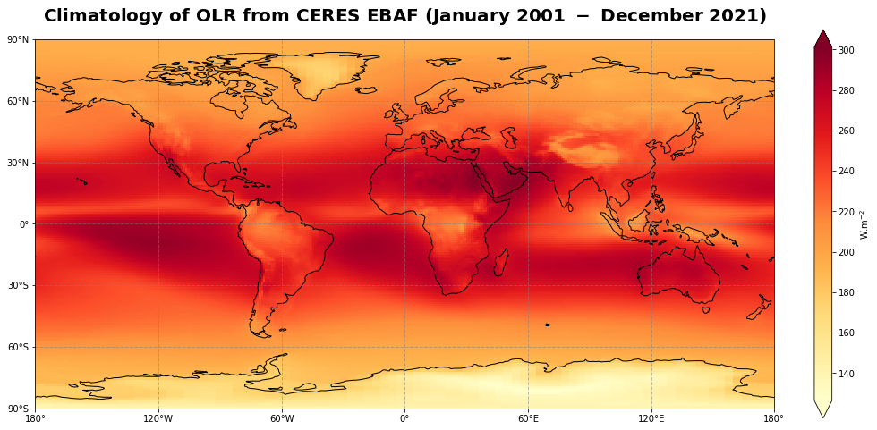
Figure 7 shows the global climatology of the top of the atmospohere outgoing longwave radiation for the time period of January 2001 - December 2021.
Time averaged seasonal climatological distribution of TOA OLR#
We now split the TOA outgoing longwave radiation data according to the seasons by using the groupby() method, with 'time.season' as an argument; the new data are then averaged over the years.
# Split data array toa_lw by season
toa_lw_seasonal_climatology = toa_lw.groupby('time.season').mean('time')
# Create a list of the seasons such as defined in the dataset toa_lw_seasonal_climatology:
seasons = ['MAM', 'JJA', 'SON', 'DJF']

# We use the "subplots" to place multiple plots according to our needs.
# In this case, we want 4 plots in a 2x2 format.
# For this "nrows" = 2 and "ncols" = 2, the projection and size are defined as well
fig8, ax8 = plt.subplots(nrows=2,
                         ncols=2,
                         subplot_kw={'projection': ccrs.PlateCarree()},
                         figsize=(16,8))

# Define a dictionary of subtitles, each one corresponding to a season
subtitles = {'MAM': 'NH spring', 'JJA': 'NH summer', 'SON': 'NH autumn', 'DJF': 'NH winter'}

# Configure the axes and subplot titles
for i_season, c_season in enumerate(seasons):
    # convert i_season index into (row, col) index
    row = i_season // 2
    col = i_season % 2
    # Plot data (coordinates and data) and define colormap
    im = ax8[row][col].pcolormesh(toa_lw_seasonal_climatology.lon,
                                  toa_lw_seasonal_climatology.lat,
                                  toa_lw_seasonal_climatology.sel(season=c_season),
                                  cmap='YlOrRd')
    # Set title and size
    ax8[row][col].set_title('Seasonal climatology of TOA LWF - ' + subtitles[c_season], fontsize=16)
    # Add coastlines
    ax8[row][col].coastlines()
    # Define grid lines and ticks (e.g. from -180 to 180 in an interval of 60)
    ax8[row][col].set_xticks(np.arange(-180, 181, 60), crs=ccrs.PlateCarree())
    ax8[row][col].set_yticks(np.arange(-90, 91, 30), crs=ccrs.PlateCarree())
    lon_formatter = LongitudeFormatter()
    lat_formatter = LatitudeFormatter()
    ax8[row][col].xaxis.set_major_formatter(lon_formatter)
    ax8[row][col].yaxis.set_major_formatter(lat_formatter)
    # Gridline
    gl = ax8[row][col].gridlines(linewidth=1, color='gray', alpha=0.5, linestyle='--')

# Place the subplots
fig8.subplots_adjust(bottom=0.0, top=0.9, left=0.05, right=0.95, wspace=0.1, hspace=0.5)

# Define and place a colorbar at the bottom
cbar_ax = fig8.add_axes([0.2, -0.1, 0.6, 0.02])
cbar = fig8.colorbar(im, cax=cbar_ax, orientation='horizontal', extend='both')
cbar.set_label('W.m$^{-2}$', fontsize=16)

# Define an overall title
fig8.suptitle('$\\bf{Seasonal\ climatology\ of\ OLR\ from\ CERES\ EBAF\ (January\ 2001\ -\ December\ 2021)}$',
              fontsize=20)

# Save the figure
fig8.savefig(f'{DATADIR}ceres_toa_lw_seasonal_climatology.png')
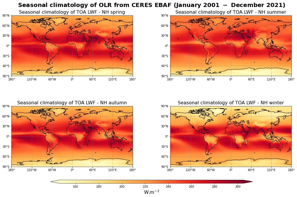
Figure 8 shows the seasonal mean climatology of the outgoing longwave flux from spring to winter (top left to bottom right panels) derived from CERES EBAF.
The general pattern is overall the same as in Figure 7 with higher values of outgoing longwave flux in the tropics and lower values in the high latitude, especially during winter. The relatively low values of OLR corresponding to high convection areas are also very well observed in the tropical summer.
Inter-annual variability of TOA OLR#
We can now analyse the inter-annual variability of the outgoing longwave radiation at the top of the atmopshere. It is defined as the root mean square of the inter-annual anomaly in the TOA OLR.
First, we apply the groupby() method to group the data array by year and calculate the time-averaged TOA OLR for each year.
# Calculate the global time-averaged distribution of TOA OLR for each year
toa_lw_clim_year = toa_lw.groupby('time.year').mean("time")
Then, we compute the inter-annual anomaly by subtracting the global mean climatology from the the group of 21 years.
# Calculate the inter-annual anomaly of TOA OLR
toa_lw_anomaly = toa_lw_clim_year - toa_lw_mean
Finally, the inter-annual variability of TOA OLR is obtained by computing the standard deviation of the anomaly.
# Calculate the inter-annual variability of TOA OLR
toa_lw_interannual_variability = toa_lw_anomaly.std("year")
# Create the figure panel and the map using the Cartopy PlateCarree projection
fig9, ax9 = plt.subplots(1, 1, figsize=(16, 8), subplot_kw={'projection': ccrs.PlateCarree()})

# Plot the data
im = plt.pcolormesh(toa_lw_interannual_variability.lon,
                    toa_lw_interannual_variability.lat,
                    toa_lw_interannual_variability,
                    cmap='YlOrRd')

# Set the figure title, add lat/lon grid and coastlines
ax9.set_title(
    '$\\bf{Interannual\ variability\ of\ TOA\ OLR\ from\ CERES\ EBAF\ (January\ 2001\ -\ December\ 2021)}$',
    fontsize=20,
    pad=20)
# Add coastlines
ax9.coastlines(color='black')
# Define gridlines and ticks
ax9.set_xticks(np.arange(-180, 181, 60), crs=ccrs.PlateCarree())
ax9.set_yticks(np.arange(-90, 91, 30), crs=ccrs.PlateCarree())
lon_formatter = LongitudeFormatter()
lat_formatter = LatitudeFormatter()
ax9.xaxis.set_major_formatter(lon_formatter)
ax9.yaxis.set_major_formatter(lat_formatter)
# Gridlines
gl = ax9.gridlines(linewidth=1, color='gray', alpha=0.5, linestyle='--')

# Specify the colorbar
cbar = plt.colorbar(im, fraction=0.025, pad=0.05, extend='both')
cbar.set_label('W.m$^{-2}$')

# Save the figure
fig9.savefig(f'{DATADIR}ceres_toa_lw_interannual_variability.png')
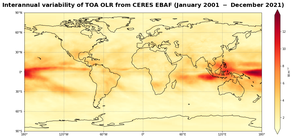
Figure 9 shows that the main variability occurs in the convective regions, in particular, in the Monsoon regions and along the Pacific Basin, following “El Niño” and “La Niña” oscillations.
Zonally averaged montly mean climatology of TOA OLR#
We will now calculate the monthly mean climatology of the outgoing longwave radiation over the time period January 2001 - December 2021 by first applying the groupby() method to group the data array by month and then calculating the average for each monthly group. The resulting data array is the monthly climatology for the total column water vapour based on reference January 2001 - December 2021.
toa_lw_clim_month = toa_lw.groupby('time.month').mean("time")
Before viewing the zonal monthly climatology of the OLR, let us average across the longitude bands with the mean() method, align the time dimension coordinate with the x axis and the lat dimension coordinate along the y axis by using the method transpose()…
toa_lw_zonal_clim_month = toa_lw_clim_month.mean(dim="lon").transpose()
Now we can plot our data. Before we do this however, we define the min, max and step of contours that we will use in a contour plot.
# Define contour parameters (min, max and step)
vdiv = 1
vmin = 100
vmax = 300
clevs = np.arange(vmin, vmax, vdiv)
# Define the figure and specify size
fig10, ax10 = plt.subplots(1, 1, figsize=(16, 8))

# Configure the axes and figure title
ax10.set_xlabel('Month')
ax10.set_ylabel('Latitude [ $^o$ ]')
ax10.set_title(
    '$\\bf{Zonally\ averaged\ monthly\ climatology\ of\ OLR\ (January\ 2001\ -\ December\ 2021)}$',
    fontsize=20,
    pad=20)

# As the months (12) are much less than the latitudes (180),
# we need to ensure the plot fits into the size of the figure.
ax10.set_aspect('auto')

# Plot the data as a contour plot
contour = ax10.contourf(toa_lw_zonal_clim_month.month,
                        toa_lw_zonal_clim_month.lat,
                        toa_lw_zonal_clim_month,
                        levels=clevs,
                        cmap='YlOrRd',
                        extend='both')
ax10.set_xticks(np.arange(1, 13, 1))
ax10.set_yticks(np.arange(-90, 91, 30))

# Specify the colorbar
cbar = plt.colorbar(contour, fraction=0.025, pad=0.05)
cbar.set_label('W.m$^{-2}$]')

# Save the figure
fig10.savefig(f'{DATADIR}ceres_toa_lw_monthly_climatology.png')
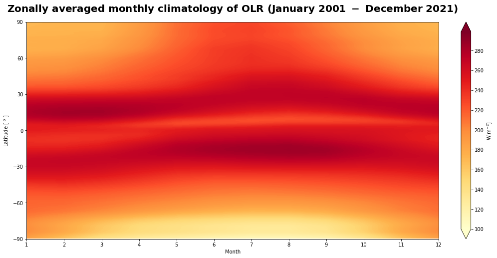
Figure 10 shows the seasonal variation of the top of the atmosphere longwave flux.
3.4. Climatology of the top-of-atmosphere net Earth’s radiation budget#
Time averaged global climatological distribution of TOA net ERB#
# Calculate the mean climatology of the net radiation at the top of the atmosphere
toa_erb_mean = solar_mean - toa_sw_mean - toa_lw_mean
We now make use of a combination of the plotting libraries Matplotlib and Cartopy to visualize the time averaged global climatological distribution of the TOA net radiative flux for the period January 2001 - December 2021.
# Create the figure panel and the map using the Cartopy PlateCarree projection
fig11, ax11 = plt.subplots(1, 1, figsize=(16, 8), subplot_kw={'projection': ccrs.PlateCarree()})

# Plot the data
im = plt.pcolormesh(toa_erb_mean.lon, toa_erb_mean.lat, toa_erb_mean, cmap='RdBu_r')

# Set the figure title, add lat/lon grid and coastlines
ax11.set_title(
    '$\\bf{Climatology\ of\ TOA\ net\ ERB\ from\ CERES\ EBAF\ (January\ 2001\ -\ December\ 2021)}$',
    fontsize=20,
    pad=20)
# Add coastlines
ax11.coastlines(color='black')
# Define gridlines and ticks
ax11.set_xticks(np.arange(-180, 181, 60), crs=ccrs.PlateCarree())
ax11.set_yticks(np.arange(-90, 91, 30), crs=ccrs.PlateCarree())
lon_formatter = LongitudeFormatter()
lat_formatter = LatitudeFormatter()
ax11.xaxis.set_major_formatter(lon_formatter)
ax11.yaxis.set_major_formatter(lat_formatter)
# Gridlines
gl = ax11.gridlines(linewidth=1, color='gray', alpha=0.5, linestyle='--')

# Specify the colorbar
cbar = plt.colorbar(im, fraction=0.025, pad=0.05, extend='both')
cbar.set_label('W.m$^{-2}$')

# Save the figure
fig11.savefig(f'{DATADIR}ceres_toa_erb_climatology.png')
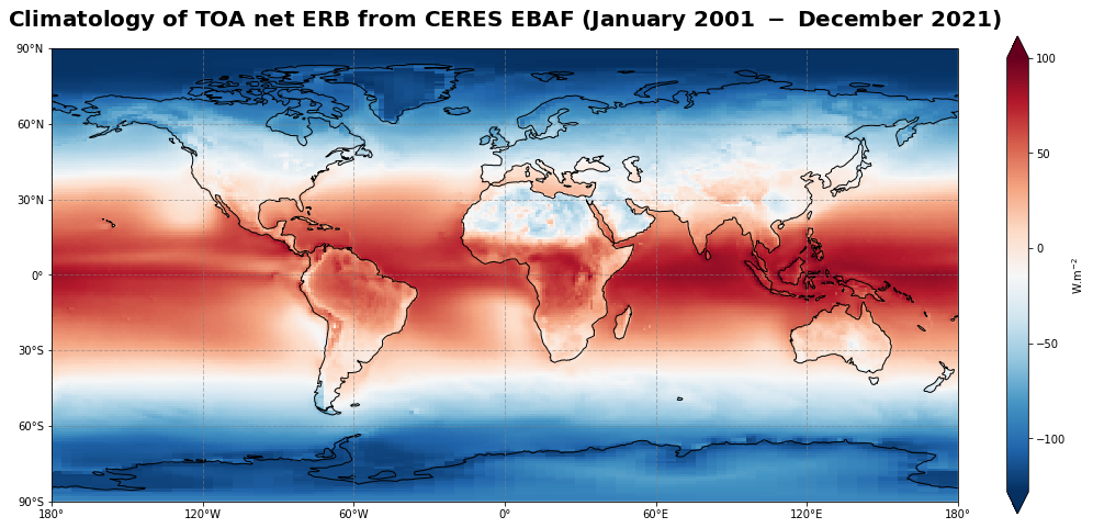
Figure 11 shows the global climatology of the (net) Earth’s radiation budget at the top of the atmosphere for the time period of January 2001 - December 2021.
Time averaged seasonal climatological distribution of TOA ERB#
To compute the time averaged seasonal climatological distribution of TOA net ERB, the data are splitted according to the seasons by using the groupby() method, with 'time.season' as an argument, and then averaged over the years.
# Select the TOA ERB data for the whole time period
toa_erb = da_toa_erb.sel(time=slice('2001-01-01', '2021-12-31'))

# Split data array TOA ERB by season
toa_erb_seasonal_climatology = toa_erb.groupby('time.season').mean('time')
# Create a list of the seasons such as defined in the dataset toa_erb_seasonal_climatology:
seasons = ['MAM', 'JJA', 'SON', 'DJF']

# We use the "subplots" to place multiple plots according to our needs.
# In this case, we want 4 plots in a 2x2 format.
# For this "nrows" = 2 and "ncols" = 2, the projection and size are defined as well
fig12, ax12 = plt.subplots(nrows=2,
                           ncols=2,
                           subplot_kw={'projection': ccrs.PlateCarree()},
                           figsize=(16,8))

# Define a dictionary of subtitles, each one corresponding to a season
subtitles = {'MAM': 'NH spring', 'JJA': 'NH summer', 'SON': 'NH autumn', 'DJF': 'NH winter'}

# Configure the axes and subplot titles
for i_season, c_season in enumerate(seasons):
    # convert i_season index into (row, col) index
    row = i_season // 2
    col = i_season % 2
    # Plot data (coordinates and data) and define colormap
    im = ax12[row][col].pcolormesh(toa_erb_seasonal_climatology.lon,
                                   toa_erb_seasonal_climatology.lat,
                                   toa_erb_seasonal_climatology.sel(season=c_season),
                                   cmap='RdBu_r')
    # Set title and size
    ax12[row][col].set_title('Seasonal climatology of TOA ERB - ' + subtitles[c_season], fontsize=16)
    # Add coastlines
    ax12[row][col].coastlines()
    # Define grid lines and ticks (e.g. from -180 to 180 in an interval of 60)
    ax12[row][col].set_xticks(np.arange(-180, 181, 60), crs=ccrs.PlateCarree())
    ax12[row][col].set_yticks(np.arange(-90, 91, 30), crs=ccrs.PlateCarree())
    lon_formatter = LongitudeFormatter()
    lat_formatter = LatitudeFormatter()
    ax12[row][col].xaxis.set_major_formatter(lon_formatter)
    ax12[row][col].yaxis.set_major_formatter(lat_formatter)
    # Gridline
    gl = ax12[row][col].gridlines(linewidth=1, color='gray', alpha=0.5, linestyle='--')

# Place the subplots
fig12.subplots_adjust(bottom=0.0, top=0.9, left=0.05, right=0.95, wspace=0.1, hspace=0.5)

# Define and place a colorbar at the bottom
cbar_ax = fig12.add_axes([0.2, -0.1, 0.6, 0.02])
cbar = fig12.colorbar(im, cax=cbar_ax, orientation='horizontal', extend='both')
cbar.set_label('W.m$^{-2}$', fontsize=16)

# Define an overall title
fig12.suptitle('$\\bf{Seasonal\ climatology\ of\ TOA\ net\ ERB\ from\ CERES\ EBAF\ (January\ 2001\ -\ December\ 2021)}$',
               fontsize=20)

# Save the figure
fig12.savefig(f'{DATADIR}ceres_toa_erb_seasonal_climatology.png')
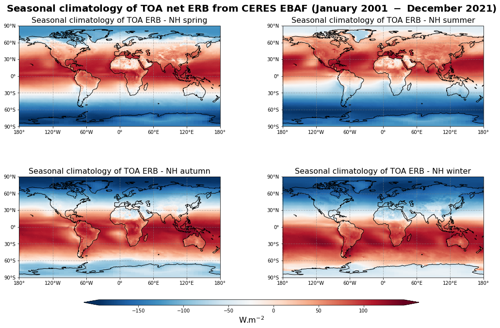
Figure 12 shows the seasonal mean climatology of the TOA net radiation from spring to winter (top left to bottom right panels) derived from CERES EBAF.
Zonally averaged montly mean climatology of TOA net ERB#
We will now calculate the monthly mean climatology of TOA net radiative flux over the period January 2001 - December 2021 by first applying the groupby() method to group the data array by month and then calculating the average for each monthly group. The resulting data array is the monthly climatology for the TOA ERB based on reference January 2001 - December 2021.
toa_erb_clim_month = toa_erb.groupby('time.month').mean("time")
Before viewing the zonal monthly climatology of the TOA ERB, we average across the longitude bands with the mean() method and align the time dimension coordinate with the x axis and the lat dimension coordinate along the y axis using the method transpose()…
toa_erb_zonal_clim_month = toa_erb_clim_month.mean(dim="lon").transpose()
Now we can plot our data. Before we do this however, we define the min, max and step of contours that we will use in a contour plot.
# Define contour parameters (min, max and step)
vdiv = 1
vmin = -200
vmax = 200
clevs = np.arange(vmin, vmax, vdiv)
# Define the figure and specify size
fig13, ax13 = plt.subplots(1, 1, figsize=(16, 8))

# Configure the axes and figure title
ax13.set_xlabel('Month')
ax13.set_ylabel('Latitude [ $^o$ ]')
# ax13.set_yticks(np.arange(-90, 91, 30))
ax13.set_title(
    '$\\bf{Zonally\ averaged\ monthly\ climatology\ of\ TOA\ net\ ERB\ (January\ 2001\ -\ December\ 2021)}$',
    fontsize=20,
    pad=20)

# As the months (12) are much less than the latitudes (180),
# we need to ensure the plot fits into the size of the figure.
ax13.set_aspect('auto')

# Plot the data as a contour plot
contour = ax13.contourf(toa_erb_zonal_clim_month.month,
                        toa_erb_zonal_clim_month.lat,
                        toa_erb_zonal_clim_month,
                        levels=clevs,
                        cmap='RdBu_r',
                        extend='both')
ax13.set_xticks(np.arange(1, 13, 1))
ax13.set_yticks(np.arange(-90, 91, 30))

# Specify the colorbar
cbar = plt.colorbar(contour, fraction=0.025, pad=0.05)
cbar.set_label('W.m$^{-2}$')

# Save the figure
fig13.savefig(f'{DATADIR}ceres_toa_erb_monthly_climatology.png')
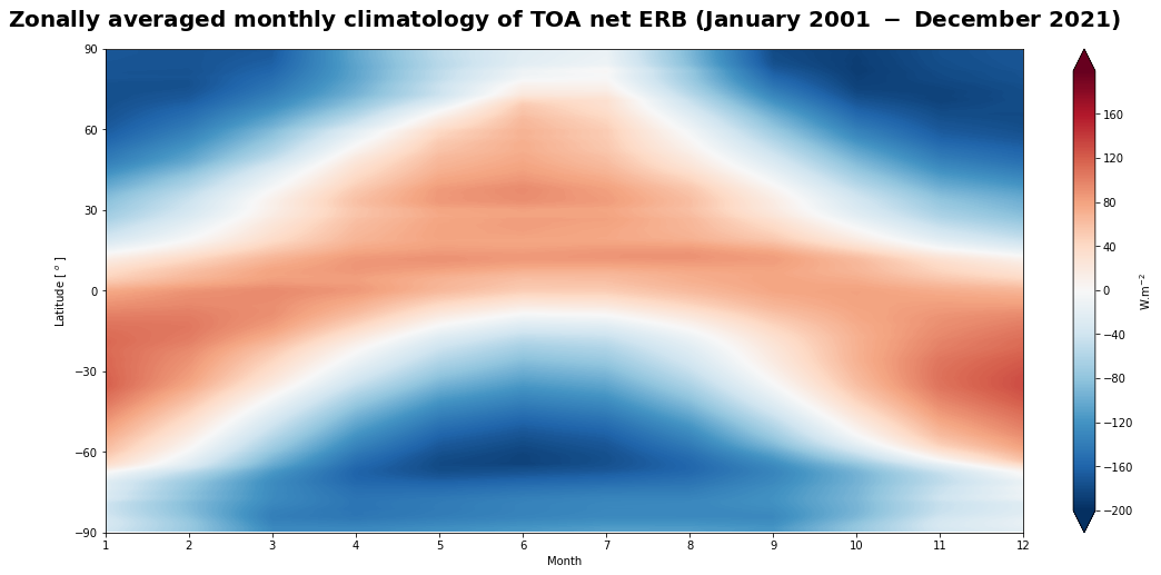
Figure 13 shows the seasonal variation of the top of atmosphere net Earth’s radiation budget.
The general pattern of the Hovmöller diagram is overall the same as the seasonal climatological distribution (Figure 12), exhibiting the oscillation of the band of positive values of TOA net ERB around the equator that reaches a maximum in the summer tropics. This confirms the dominant effect of the solar radiation and the equator-versus-pole energy imbalance which is the main driver of atmospheric and oceanic circulations.
4. Time series and trend analysis of the Earth’s Radiation Budget#
We first create a temporal subset for the time period January 2001 to December 2021.
# Select time period for the incoming shortwave radiation data array
ceres_solar = da_solar.sel(time=slice('2001-01-01', '2021-12-31'))

# Select time period for the outgoing shortwave radiation data array
ceres_toa_sw = da_toa_sw.sel(time=slice('2001-01-01', '2021-12-31'))

# Select time period for the outgoing longwave radiation data array
ceres_toa_lw = da_toa_lw.sel(time=slice('2001-01-01', '2021-12-31'))

# Compute the net radiative flux for the selected time period
ceres_toa_erb = ceres_solar - ceres_toa_sw - ceres_toa_lw
Spatial aggregation#
# Define weights as the cosine of latitudes
weights = np.cos(np.deg2rad(ceres_solar.lat))
weights.name = "weights"

# Spatial aggregation of CERES-EBAF incident solar flux
ceres_solar_weighted = ceres_solar.weighted(weights)

# Spatial aggregation of CERES-EBAF reflected solar flux
ceres_toa_sw_weighted = ceres_toa_sw.weighted(weights)

# Spatial aggregation of CERES-EBAF Earth emitted longwave flux
ceres_toa_lw_weighted = ceres_toa_lw.weighted(weights)

# Spatial agregation of CERES-EBAF net radiative flux
ceres_toa_erb_weighted = ceres_toa_erb.weighted(weights)
The next step is to compute the mean across the latitude and longitude dimensions of the weighted data array with the mean() method.
# Weighted mean of CERES-EBAF incident solar flux
ceres_solar_wmean = ceres_solar_weighted.mean(dim=("lat", "lon"))

# Weighted mean of CERES-EBAF reflected solar flux
ceres_toa_sw_wmean = ceres_toa_sw_weighted.mean(dim=("lat", "lon"))

# Weighted mean of CERES-EBAF Earth emitted longwave flux
ceres_toa_lw_wmean = ceres_toa_lw_weighted.mean(dim=("lat", "lon"))

# Weighted mean of CERES net radiative flux
ceres_toa_erb_wmean = ceres_toa_erb_weighted.mean(dim=("lat", "lon"))
4.1. Time series and trend analysis of the top-of-atmosphere incoming solar radiation#
Global time series of TIS#
Now we can plot the time series of globally averaged TIS data over time using the plot() method.
# Define the figure and specify size
fig14, ax14 = plt.subplots(1, 1, figsize=(16, 8))

# Configure the axes and figure title
ax14.set_xlabel('Year')
ax14.set_ylabel('W.m$^{-2}$')
ax14.grid(linewidth=1, color='gray', alpha=0.5, linestyle='--')
ax14.set_title('$\\bf{Global\ time\ series\ of\ TIS\ from\ CERES\ EBAF}$', fontsize=20, pad=20)

# Plot the data
ax14.plot(ceres_solar_wmean.time, ceres_solar_wmean)

# Save the figure
fig14.savefig(f'{DATADIR}ceres_isf_global_timeseries.png')
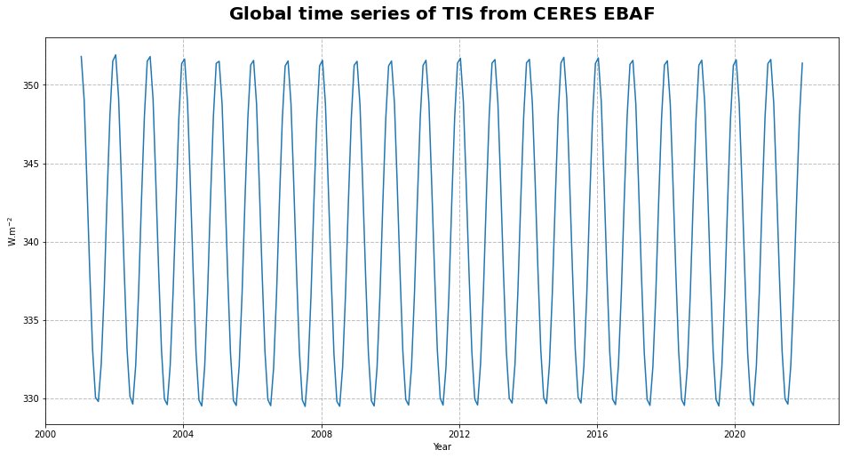
Figure 14 shows the time series of the incoming solar flux at the top of the atmosphere.
Trend analysis and seasonal cycle of TIS#
The time series can be further analysed by extracting the trend, or the running annual mean, and the seasonal cycle.
To this end, we will convert the Xarray Data Array into a time series with the pandas library before decomposing it into the trend, the seasonal cycle and the residuals by using the seasonal_decompose() method and visualizing the results.
# Convert the Xarray data array ceres_solar_wmean into a time series
ceres_solar_wmean_series = pd.Series(ceres_solar_wmean)
# Define the time dimension of ceres_solar_weighted_mean as the index of the time series
ceres_solar_wmean_series.index = ceres_solar_wmean.time.to_dataframe().index

# Decomposition of the time series into the trend, the seasonal cycle and the residuals
ceres_solar_seasonal_decomposition = seasonal_decompose(ceres_solar_wmean_series,
                                                        model='additive',
                                                        period=12)

# Plot the resulting seasonal decomposition
ceres_solar_seasonal_decomposition.plot()
plt.xlabel("Time")
plt.savefig(f'{DATADIR}ceres_solar_timeseries_climatology.png')
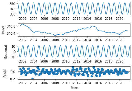
Figure 15 shows the decomposition of the TIS time series into the trend corresponding to the sunspot cycle (2nd panel), and the seasonal cycle with the confirmed amplitude of 20 W/m\(^{2}\) (3rd panel), from which are derived the anomalies or de-trended and de-seasonalised time series that have the characteristics of an uncorrelated noise pattern (4th panel).
4.2. Time series and trend analysis of the top-of-atmosphere reflected solar flux#
Global time series of TOA RSF#
We will now plot the time series of globally averaged TOA RSF data over time using the plot() method.
# Define the figure and specify size
fig16, ax16 = plt.subplots(1, 1, figsize=(16, 8))

# Configure the axes and figure title
ax16.set_xlabel('Year')
ax16.set_ylabel('W.m$^{-2}$')
ax16.grid(linewidth=1, color='gray', alpha=0.5, linestyle='--')
ax16.set_title('$\\bf{Global\ time\ series\ of\ TOA\ RSF\ from\ CERES\ EBAF}$', fontsize=20, pad=20)

# Plot the data
ax16.plot(ceres_toa_sw_wmean.time, ceres_toa_sw_wmean)

# Save the figure
fig16.savefig(f'{DATADIR}ceres_toa_sw_global_timeseries.png')
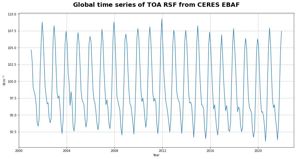
Figure 16 shows the time series of the reflected solar flux at the top of the atmosphere.
From the time series of the global space and time averaged RSF, we can infer a clear seasonal cycle associated to the Earth’s orbit around the sun and a long-term seasonal cycle corresponding to the sunspot cycle together with a negative trend. They will now be further examined through the seasonal decomposition of the incoming solar flux.
Trend analysis and seasonal cycle of TOA RSF#
The time series can be further analysed by extracting the trend, or the running annual mean, and the seasonal cycle.
To this end, we will convert the Xarray Data Array into a time series with the pandas library before decomposing it into the trend, the seasonal cycle and the residuals by using the seasonal_decompose() method and visualizing the results.
# Convert the Xarray data array ceres_toa_sw_wmean into a time series
ceres_toa_sw_wmean_series = pd.Series(ceres_toa_sw_wmean)
# Define the time dimension of ceres_toa_sw_wmean as the index of the time series
ceres_toa_sw_wmean_series.index = ceres_toa_sw_wmean.time.to_dataframe().index

# Decomposition of the time series into the trend, the seasonal cycle and the residuals
ceres_toa_sw_seasonal_decomposition = seasonal_decompose(ceres_toa_sw_wmean_series,
                                                         model='additive',
                                                         period=12)

# Plot the resulting seasonal decomposition
ceres_toa_sw_seasonal_decomposition.plot()
plt.xlabel("Time")
plt.savefig(f'{DATADIR}ceres_toa_sw_timeseries_climatology.png')
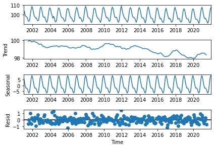
Figure 17 shows the decomposition of the TOA RSF time series into a negative trend of ~-0.1 W/m\(^{2}\)/year (2nd panel) and a seasonal cycle with an amplitude of ~15 W/m\(^{2}\) (3rd panel), from which are derived the anomalies that have the characteristics of an uncorrelated noise pattern (4th panel).
4.3. Time series and trend analysis of the top-of-atmosphere outgoing longwave radiation#
Global time series of TOA OLR#
We will now plot the time series of globally averaged outgoing longwave radiation data over time using the plot() method.
# Define the figure and specify size
fig18, ax18 = plt.subplots(1, 1, figsize=(16, 8))

# Configure the axes and figure title
ax18.set_xlabel('Year')
ax18.set_ylabel('W.m$^{-2}$')
ax18.grid(linewidth=1, color='gray', alpha=0.5, linestyle='--')
ax18.set_title('$\\bf{Global\ time\ series\ of\ OLR\ from\ CERES\ EBAF}$', fontsize=20, pad=20)

# Plot the data
ax18.plot(ceres_toa_lw_wmean.time, ceres_toa_lw_wmean)

# Save the figure
fig18.savefig(f'{DATADIR}ceres_toa_lw_global_timeseries.png')
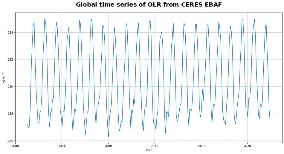
Figure 18 shows the time series of the outgoing longwave radiation at the top of the atmosphere. From the time series, we can infer a seasonal pattern along with a trend in the global space and time averaged TOA OLR.
We will now procede to the seasonal decomposition of the Earth-emitted longwave radiation at the top of the atmosphere and analyse more specifically the trend and seasonal cycle of CERES-EBAF OLR.
Trend analysis and seasonal cycle of TOA OLR#
The time series can be further analysed by extracting the trend, or the running annual mean, and the seasonal cycle.
To this end, we will convert the Xarray Data Array into a time series with the pandas library before decomposing it into the trend, the seasonal cycle and the residuals by using the seasonal_decompose() method and visualizing the results.
# Convert the Xarray data array ceres_toa_lw_wmean into a time series
ceres_toa_lw_wmean_series = pd.Series(ceres_toa_lw_wmean)
# Define the time dimension of ceres_toa_lw_wmean as the index of the time series
ceres_toa_lw_wmean_series.index = ceres_toa_lw_wmean.time.to_dataframe().index

# Decomposition of the time series into the trend, the seasonal cycle and the residuals
ceres_toa_lw_seasonal_decomposition = seasonal_decompose(ceres_toa_lw_wmean_series,
                                                         model='additive',
                                                         period=12)

# Plot the resulting seasonal decomposition
ceres_toa_lw_seasonal_decomposition.plot()
plt.xlabel("Time")
plt.savefig(f'{DATADIR}ceres_toa_lw_timeseries_climatology.png')
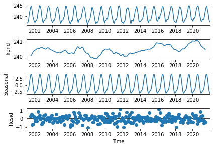
Figure 19 shows the decomposition of the outgoing lonwave radiation time series into a positive trend of ~0.05 W/m\(^{2}\)/year (2nd panel), and a seasonal cycle with an amplitude of ~8 W/m\(^{2}\) (3rd panel), from which are derived the anomalies that have the characteristics of uncorrelated noise pattern (4th panel).
The observed inter-annual variations in the 2nd panel of Figure 19 suggest an influence of the “El Niño” or “La Niña” Southern Oscillation on the TOA OLR. The increase in this Earth-emitted longwave radiation is clearly related to the increase of surface temperatures.
4.4. Time series and trend analysis of the top-of-atmosphere net Earth’s radiation budget#
Global time series of TOA net ERB#
We will now plot the time series of the globally averaged TOA net Earth’s radiative flux over time using the plot() method.
# Define the figure and specify size
fig20, ax20 = plt.subplots(1, 1, figsize=(16, 8))

# Configure the axes and figure title
ax20.set_xlabel('Year')
ax20.set_ylabel('W.m$^{-2}$')
ax20.grid(linewidth=1, color='gray', alpha=0.5, linestyle='--')
ax20.set_title('$\\bf{Global\ time\ series\ of\ TOA\ net\ ERB\ from\ CERES\ EBAF}$', fontsize=20, pad=20)

# Plot the data
ax20.plot(ceres_toa_erb_wmean.time, ceres_toa_erb_wmean)

# Save the figure
fig20.savefig(f'{DATADIR}ceres_toa_erb_global_timeseries.png')
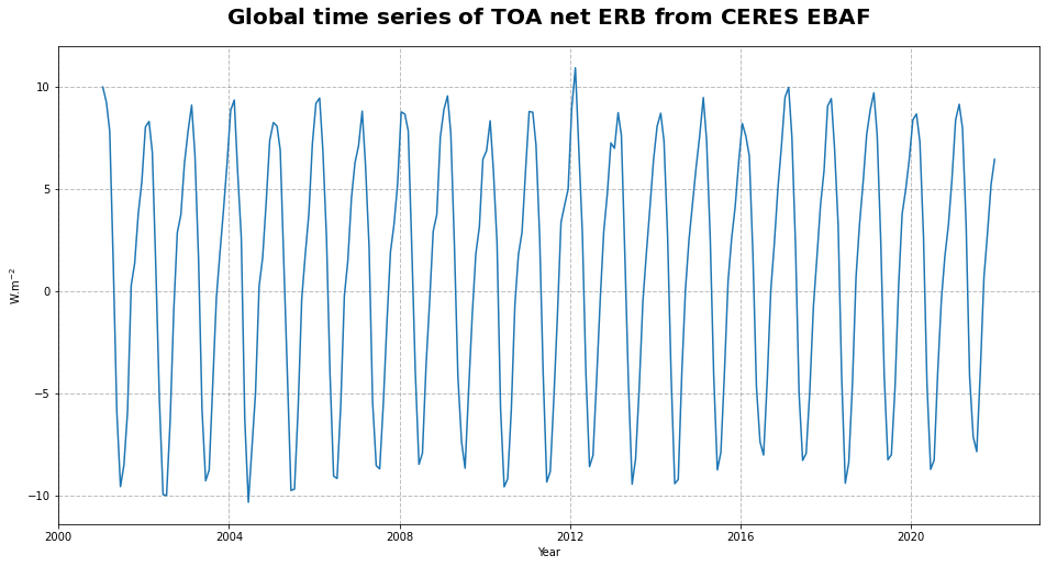
Figure 20 shows the time series of the net Earth’s radiation budget at the top of the atmosphere. From the time series, we can infer a seasonal pattern together with a slightly increasing trend in the global space and time averaged TOA net ERB.
Trend analysis and seasonal cycle of TOA net ERB#
The time series can be further analysed by extracting the trend, or the running annual mean, and the seasonal cycle.
# Convert the Xarray data array ceres_toa_erb_wmean into a time series
ceres_toa_erb_wmean_series = pd.Series(ceres_toa_erb_wmean)
# Define the time dimension of ceres_toa_sw_wmean as the index of the time series
ceres_toa_erb_wmean_series.index = ceres_toa_erb_wmean.time.to_dataframe().index

# Decomposition of the time series into the trend, the seasonal cycle and the residuals
ceres_toa_erb_seasonal_decomposition = seasonal_decompose(ceres_toa_erb_wmean_series,
                                                          model='additive',
                                                          period=12)

# Plot the resulting seasonal decomposition
ceres_toa_erb_seasonal_decomposition.plot()
plt.xlabel("Time")
plt.savefig(f'{DATADIR}ceres_toa_erb_timeseries_climatology.png')
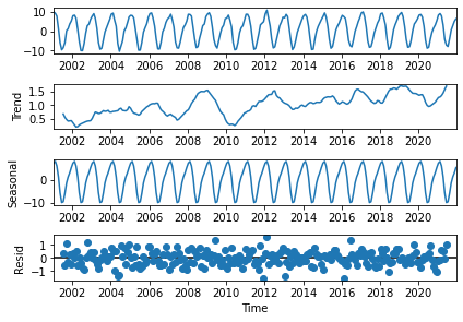
Figure 21 shows the decomposition of the CERES-EBAF TOA net ERB time series into a positive trend of ~0.05 W/m\(^{2}\)/year (2nd panel), and a seasonal cycle with an amplitude of ~20 W/m\(^{2}\) (3rd panel), from which are derived the anomalies that have the characteristics of uncorrelated noise pattern (4th panel).