Tutorial: Visualising Lake Water Level (LWL) timeseries

Tutorial: Visualising Lake Water Level (LWL) timeseries#

Before continuing with this tutorial, please verify that the C3S API is installed. All the information about this api is available at:

https://cds.climate.copernicus.eu/api-how-to#install-the-cds-api-key

In this tutorial we will access lake products from the Climate Data Store (CDS) and analyse the timeseries of the lake water level on a selected lake. The tutorial comprises two main steps:

Dowload and decompress data
Visualise the location of the lake in a map
Visualise and save water level timeseries
Visualise and save the yearly water level anomalies

Import librairies#

The lake water level data will be download in a zip file containing a NetCDF file. We need libraries to download data from the CDS but also libraires to manage zip files (zipfile library) and NetCDF files (xarray library). We also use libraries to plot and visualise data (matplotlib and cartopy libraries).

Additional libraires: os and glob are used for file management

# If necessary install the dependant libraries, this cell need only be run once:
!pip install -q cdsapi
!pip install -q xarray
!pip install -q matplotlib cartopy

import cdsapi
import os
import glob
import zipfile
import xarray as xr
import numpy as np
import matplotlib.pyplot as plt
from cartopy import crs, feature

Set up an output directory to store data and plots#

# the output directory name 
output_dir = 'output'

# The output directory must exitst. If it is not the case, it must be created. 
if os.path.exists(output_dir) == False:
    os.makedirs(output_dir)

2. Visualise lake location#

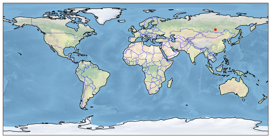
It is always a useful idea to check the lake’s location on a map. Many of the world’s lakes have the same name but may be located in different countries, as in the case of Lake Victoria: the best known is in Uganda, but there is also a Lake Victoria in Canada (48.35N, 57.11W) and another in Australia (34.04S, 141.28E). Or the name of the lake is different, depending on the language: Caribou Lake or Rendeer lake refer to the same lake (Canada). In some cases, even with the same language, lake name can differ between countries: Lake Buenos Aires in Argentina and Lake General Carrera in Chili.

A world map, with the location of the lake is displayed. For generating this figure we use the cartopy library.

fig = plt.figure(figsize = (12,6))
ax = plt.subplot(1,1,1, projection = crs.PlateCarree())

ax.coastlines()
ax.add_feature(feature.BORDERS, linewidth=0.5, edgecolor='blue')
ax.stock_img()

# add lake location 
lat = float(xr_lake.lake_barycentre_latitude.split()[0])
if 'S' in xr_lake.lake_barycentre_latitude:
    lat = -lat
lon = float(xr_lake.lake_barycentre_longitude.split()[0])
if 'W' in xr_lake.lake_barycentre_longitude:
    lon = -lon
    
print (f"Lake location (lat, lon): {lat}°, {lon}°")
plt.scatter(x = [lon], y = [lat], s = 30, color = 'red', transform = crs.PlateCarree())

Lake location (lat, lon): 53.58°, 108.17°

<matplotlib.collections.PathCollection at 0x162889cc0>

../../_images/d733abffa611be0039cf3097c7d10914883146fe2261d5b8746bacf43d34b058.png

3. Visualise lake water level time series#

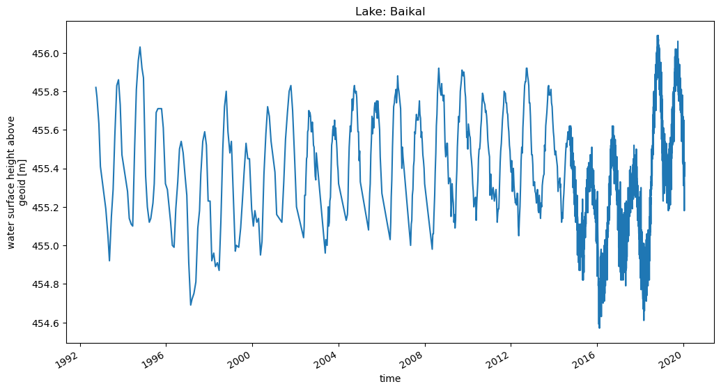
Now that the data has been extracted, we can read it and plot it. To read the data in NetCDF format we use the Xarray library and for the visualisation of the time series we use Matplotlib

The figure with the timeseries will be saved in the output directory in png format: [lake_name]_timeseries.png file

The change in time step due to coverage by multiple missions can be seen in the figure: in recent years, Lake Baikal has been monitored by multiple missions and trajectories. As a result, the temporal resolution increases (the time between observations is reduced) and the time series is noisier due to the effect of the inter-mission and inter-tracks bias.

# plot and visualise the timeseries
fig = plt.figure(figsize = (12, 6))
xr_lake.water_surface_height_above_reference_datum.plot()
plt.title(f'Lake: {lake_name.title()}')

# save the figure
png_file = f'{output_dir}/{lake_name}_timeseries.png'
plt.savefig(png_file, dpi=300, bbox_inches="tight")

../../_images/f5c1c111b171fc11a1133a9e1bb5959c51797a3cc3eae29918944172e029bbac.png

3. Visualise lake water level yearly anomalies#

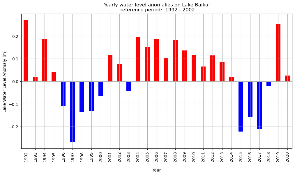
Another way of analysing variations in water levels is to visualise anomalies in relation to average values over a reference period in the form of a bar chart, using red and blue colours to easily identify the year when levels are higher or lower than the climatic normal.

The same code can be used for the visualiation of yearly anomalies compared to a particular year.

The reference period can be adapted to each lake. Indeed, the temporal coverage is not the same for all the lakes in the CDS, with the first available date ranging from 1992, as is the case for Lake Baikal, to 2019 for lakes monitored exclusively by the Sentinel-3B mission. In this example for Lake Baikal, we have chosen a reference period consisting of the first 10 years of data.

first_reference_year = 1992
last_reference_year  = 2002

The yearly anomaly is calculated by first applying xarray’s groupby() function to group the data by year and then calculating the mean value for each annual group. The average value of the water in the reference lake is estimated as the average water level over the reference period.

yearly_mean = xr_lake.groupby('time.year').mean(keep_attrs = True)

ref = yearly_mean.where((yearly_mean.year >= first_reference_year ) & (yearly_mean.year <= last_reference_year ))
ref_lwl_mean = np.nanmean(ref.water_surface_height_above_reference_datum.values)

print (f'Mean LWL value during the reference period: {np.round(ref_lwl_mean,3)} (m)')

Mean LWL value during the reference period: 455.386 (m)

The yearly anomaly is shown in red for values above the average water level during the reference period and in blue for values below.

The figure with the anomalies is saved in the output directory in png format : [lake_name]_yearly-anomalies.png file

year_mean = yearly_mean.to_dataframe()
year_mean['lwl_yearly_anomaly'] = year_mean['water_surface_height_above_reference_datum'] - ref_lwl_mean
year_mean['positive_anomaly'] = year_mean['lwl_yearly_anomaly'] > 0

fig, ax = plt.subplots(figsize=(12, 6))
year_mean['lwl_yearly_anomaly'].plot(kind='bar', 
                                     color = year_mean.positive_anomaly.map ({True: 'red', False: 'blue'}),
                                     xlabel = '\nYear',
                                     ylabel = 'Lake Water Level Anomaly (m)',
                                     title = f'Yearly water level anomalies on Lake {lake_name.title()}\n reference period:  {first_reference_year} - {last_reference_year}')

ax.grid()

# save the figure
png_file = f'{output_dir}/{lake_name}_yearly-anomalies.png'
plt.savefig(png_file, dpi=300, bbox_inches='tight')

../../_images/97529ea9cd212a7c263c12cd0559b57d237bb664cefdb4952712b1b4958cdb1e.png

Tutorial: Visualising Lake Water Level (LWL) timeseries

Contents

Tutorial: Visualising Lake Water Level (LWL) timeseries#

Import librairies#

Set up an output directory to store data and plots#

Lake selection#

1. Dowload and decompress data#

2. Visualise lake location#

3. Visualise lake water level time series#

3. Visualise lake water level yearly anomalies#