Greenland Ice Sheet velocity

Greenland Ice Sheet velocity#

By J. Wuite, ENVEO IT GmbH, jan.wuite@enveo.at

About#

This tutorial will demonstrate how to plot velocity maps and flow vectors of the Greenland Ice Sheet and its major outlet glaciers, using ice velocity data from the Copernicus Climate Change Service (C3S).

It will show you how to download data from the C3S Climate Data Store (CDS), plot the maps and and display flow vectors on top.

Prepare your environment#

To download data from the CDS, you must complete three steps;

Register for free with the CDS at https://cds.climate.copernicus.eu/#!/home
Set up the CDS Application Program Interface (API), as described at https://cds.climate.copernicus.eu/api-how-to
Agree to the dataset terms of use - if you have not already done so you will be directed to the correct webpage the first time you try to download data. Accept the terms and conditions, and re-run the downloading code.

Import libraries#

The data is stored in netCDF4 files. To work with them, several libraries are needed. These are used to retrieve the data, unpack it, run calculations and plot the results.

# CDS API
import cdsapi

# File handling
import shutil
import glob
import os

# Calculations
import numpy as np
import xarray as xr

# Mapping
import cartopy.crs as ccrs

# Plotting
import matplotlib.pyplot as plt

Download data#

Select the ice sheet of interest (currently only Greenland) and retrieve the dataset. An example of how to retrieve the data is given on the CDS, under ‘Show API request’ on the dataset’s webpage at https://cds.climate.copernicus.eu/cdsapp#!/dataset/satellite-greenland-ice-sheet-velocity?tab=form

The dataset comes in a zip file, and may takesome time to load (>650 Mb).

# Set ice_sheet to the desired ice sheet, either 'greenland' or 'antarctica' (not active yet) and select year/version
# This will be used to select data, and later to set up plot defaults

ice_sheet = 'greenland'
year = '2020_2021'
version = '1.4'

# Download data from the CDS
dataset='satellite-%s-ice-sheet-velocity' % ice_sheet

c = cdsapi.Client()

c.retrieve(
    dataset,
    {
        'period': year,
        'version': version,
        'variable': 'all',
        'format': 'zip',
    },
    'download.zip')

# Unpack the zip file and remove the zipped data

shutil.unpack_archive('download.zip', '.')
os.remove('download.zip')

# List the files contained and select the latest netCDF (.nc) file. Print its filename

list_of_files = glob.glob('*.nc') # * means all if need specific format then *.nc
latest_file = max(list_of_files, key=os.path.getctime)
print('In the following you are seeing the data from: \n'+latest_file)

2024-01-15 12:22:56,163 INFO Welcome to the CDS
2024-01-15 12:22:56,164 INFO Sending request to https://cds.climate.copernicus.eu/api/v2/resources/satellite-greenland-ice-sheet-velocity
2024-01-15 12:22:56,315 INFO Request is completed
2024-01-15 12:22:56,315 INFO Downloading https://download-0012-clone.copernicus-climate.eu/cache-compute-0012/cache/data2/dataset-satellite-greenland-ice-sheet-velocity-851a38ea-6ff0-49ea-8fca-84d5b7b38b4e.zip to download.zip (663M)
2024-01-15 12:24:37,394 INFO Download rate 6.6M/s                                                                                                                                        

In the following you are seeing the data from: 
C3S_GrIS_IV_250m_S1_20201001_20210930_v1_4.nc

Examine the data#

Open the data file and list its contents. These include descriptive comments.

# Open the NetCDF file

ds = xr.open_dataset(latest_file)

# Print contents list

print('The data file contains the following:')
print(ds)

The data file contains the following:
<xarray.Dataset>
Dimensions:                              (y: 10801, x: 5984)
Coordinates:
  * y                                    (y) float64 -6.556e+05 ... -3.356e+06
  * x                                    (x) float64 -6.399e+05 ... 8.559e+05
Data variables:
    crs                                  int32 ...
    land_ice_surface_easting_velocity    (y, x) float32 ...
    land_ice_surface_northing_velocity   (y, x) float32 ...
    land_ice_surface_vertical_velocity   (y, x) float32 ...
    land_ice_surface_velocity_magnitude  (y, x) float32 ...
    land_ice_surface_measurement_count   (y, x) float64 ...
    land_ice_surface_easting_stddev      (y, x) float32 ...
    land_ice_surface_northing_stddev     (y, x) float32 ...
Attributes: (12/13)
    Conventions:    CF-1.7
    title:          Ice Velocity of the Greenland Ice Sheet
    reference:      Main: Nagler, T.; Rott, H.; Hetzenecker, M.; Wuite, J.; P...
    source:         Copernicus Sentinel-1A and Sentinel-1B
    institution:    Copernicus Climate Change Service
    contact:        copernicus-support@ecmwf.int
    ...             ...
    creation_date:  2022-12-12
    comment:        Ice velocity map of Greenland derived from Sentinel-1 SAR...
    history:        product version 1.4
    summary:        Ice velocity derived for Greenland Ice Sheet gridded at 2...
    keywords:       EARTH SCIENCE CLIMATE INDICATORS CRYOSPHERIC INDICATORS G...
    license:        C3S general license

/usr/lib64/python3.11/site-packages/numpy/core/getlimits.py:518: UserWarning: The value of the smallest subnormal for <class 'numpy.float64'> type is zero.
  setattr(self, word, getattr(machar, word).flat[0])
/usr/lib64/python3.11/site-packages/numpy/core/getlimits.py:89: UserWarning: The value of the smallest subnormal for <class 'numpy.float64'> type is zero.
  return self._float_to_str(self.smallest_subnormal)
/usr/lib64/python3.11/site-packages/numpy/core/getlimits.py:518: UserWarning: The value of the smallest subnormal for <class 'numpy.float32'> type is zero.
  setattr(self, word, getattr(machar, word).flat[0])
/usr/lib64/python3.11/site-packages/numpy/core/getlimits.py:89: UserWarning: The value of the smallest subnormal for <class 'numpy.float32'> type is zero.
  return self._float_to_str(self.smallest_subnormal)

Plot the Greenland Ice Sheet velocity map and display flowvectors on top#

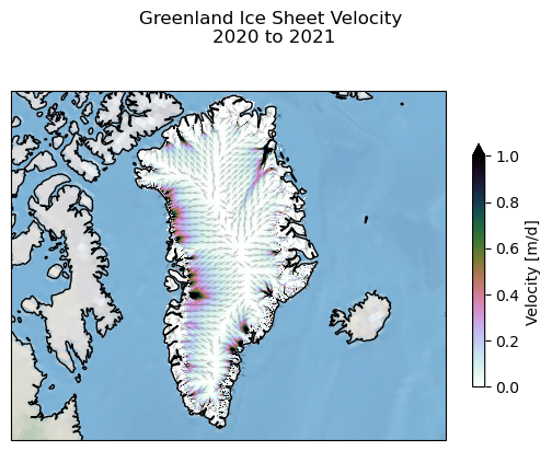
The dataset contains annual ice velocity maps of the Greenland Ice Sheet derived from Sentinel-1 data. The data represent the current state-of-the-art in Europe for production of satellite-based ice velocity data records. It follows on from the ESA Greenland Ice Sheet Climate Change Initiative and is guided by the GCOS (Global Climate Observing System) targets for the Ice Sheets Essential Climate Variable.

Mapping glacier flow velocity and its temporal changes provides key information for investigating the dynamic response of glaciers and ice sheets to changing boundary environmental conditions. Remote sensing techniques that utilise satellite data are the only feasible manner to derive accurate surface velocities of the remote Greenland glaciers on a regular basis.

The surface velocity is derived by applying feature tracking techniques using Sentinel-1 synthetic aperture radar (SAR) data acquired in the Interferometric Wide (IW) swath mode. Ice velocity is provided at 250m and 500m grid spacing in North Polar Stereographic projection (depending on version). The horizontal velocity components are provided in true meters per day, towards easting and northing direction of the grid. The vertical displacement is derived from a digital elevation model. Provided is a NetCDF file with the velocity components: vx, vy, vz, along with maps showing the magnitude of the horizontal components, the valid pixel count and uncertainty (based on the standard deviation). The product combines all ice velocity maps, based on 6- and 12-day repeats, acquired over a full year in an annually averaged product running from October 1st to September 30th, mimicking a glaciological year. The dataset is extended on an annual basis.

This dataset is produced on behalf of the Copernicus Climate Change Service (C3S).

# Plot the ice velocity map in a figure in Polar Stereographic projection with a nice background, color map and vectors on top

#For Greenland:

projection = ccrs.NorthPolarStereo(central_longitude=-45, true_scale_latitude=70) #EPSG:3413
ext = [-73, -12, 59, 83]    # map boundaries, in degrees, [east, west, south, north]
    
# Create a new figure

fig = plt.figure()
title='Greenland Ice Sheet Velocity \n'+year[0:4]+ ' to ' +year[5:9]
fig.suptitle(title, fontsize=12)

# Add a new subplot to the figure with the projection defined above


ax = plt.axes(projection=projection)

# Set the extent of the map to the longitude and latitude range defined above

ax.set_extent(ext, crs=ccrs.PlateCarree())

# Add a background image and coastlines to the map
ax.stock_img()
ax.coastlines(resolution='50m')

# Plot the velocity magnitude data on the map. Customise the plot settings.

vmin=0        # Values below this value will be set to the bottom of the colour range
vmax=1          # Values above this value will be set to the top of the colour range
cmap='cubehelix_r'      # Reversed cubehelix colortable 

ds.land_ice_surface_velocity_magnitude.plot(vmin=vmin, vmax=vmax, cmap=cmap,cbar_kwargs={'label': "Velocity [m/d]",'shrink': 0.6})

# Extract the easting and northing velocity and display a selection on top as flow vectors

u=ds.land_ice_surface_easting_velocity.values
v=ds.land_ice_surface_northing_velocity.values
y=ds.coords['y'].values
x=ds.coords['x'].values

X=[]
Y=[]
U=[]
V=[]

for yi in range(0, u.shape[0], 200):
  for xi in range(0, u.shape[1], 200):
    X.append(x[xi])
    Y.append(y[yi])
    # Normalize to display all vectors at same length:
    U1=u[yi][xi]
    V1=v[yi][xi]
    U.append(U1 / np.sqrt(U1**2 + V1**2)) 
    V.append(V1 / np.sqrt(U1**2 + V1**2))
    scale=50
    # For proportionate vector length comment the above section and uncomment the following instead:
    #U.append(u[yi][xi])
    #V.append(v[yi][xi])
    #scale=5
plt.quiver(X,Y,U,V,scale=scale,alpha=0.2,color="black")

# Display the plot

plt.show()

../../_images/b1d55792e6887e573df41f69fbfedcdfb72113f3be5298cf277c5a7fc9ab68fa.png

Zoom into key outlet glaciers of the Greenland Ice Sheet#

The following zooms into some of the biggest outlet glaciers of the Greenland Ice Sheet and plots the ice velocity in subplots using a different color code.

import cartopy.crs as ccrs
projection = ccrs.NorthPolarStereo(central_longitude=-45, true_scale_latitude=70) #EPSG:3413

extents = {
    #'Hagen Glacier': [-33, -27, 81, 81.6],
    'Helheim Glacier': [-40, -37, 66, 67],
    #'Illullip Sermia': [-56.5, -55, 74.2, 74.6],
    'Jakobshavn Isbræ': [-51, -46, 68.5, 70.5],
    'Kangerlussaq Glacier': [-36, -32, 68, 70],
    'Petermann Glacier': [-62, -55, 80, 81.5],
    'Rink Glacier': [-53, -47, 71, 72.5],
    #'Ryder Glacier': [-53, -47, 80.5, 82],
    'Zachariae Isstrom': [-30, -20, 78, 80]
} # map boundaries for ke glaciers, in degrees, [east, west, south, north]

title='Greenland Ice Sheet Velocity 2020-2021'
fig = plt.figure()
fig.suptitle(title, fontsize=12)
fig, axs = plt.subplots(nrows=2, ncols=3, subplot_kw={'projection': projection})
axs = axs.flatten()

i=0
for x in extents:
  axs[i].set_extent(extents[x], crs=ccrs.PlateCarree())
  axs[i].stock_img()
  axs[i].coastlines(resolution='50m')
  ds.land_ice_surface_velocity_magnitude.plot(ax=axs[i],vmin=0, vmax=2, cmap='viridis', cbar_kwargs={'label': "m/d",'shrink': 0.6})
  axs[i].set_title(x)    
  i+=1

plt.show()