Tutorial on how to import, subset, aggregate and export CAMS Data

This tutorial provides practical examples that demonstrate how to download, read into Xarray, subset, aggregate and export data from the Atmosphere Data Store (ADS) of the Copernicus Atmosphere Monitoring Service (CAMS).

---

Learning objectives 🧠

1. Understanding what are multidimensional arrays and what are they used for.

2. Learning to read and export multidimensional arrays with the Python library xarray: familiarizing with the netCDF format and the temporal and geographical dimensions of the CAMS data.

3. Learning how multidimensional arrays can be subsetted and aggregated using xarray: practicing different ways to subset and aggregate according to time and space.

---

Target audience 🎯

Anyone interested in accessing, manipulating and using data from the Copernicus Atmosphere Data Store (ADS).

---

Prerequisites and assumed knowledge 🔍

1. Basic Programming Skills: Familiarity with programming concepts, particularly in Python, as the tutorial involves using Python libraries like xarray for dealing with multidimensional arrays.

2. Familiarity with API Usage: Understanding of how to use Application Programming Interfaces (APIs) will be useful for accessing data through the CDS API.

3. Familiarity with multidimensional data structure: Comprehending what are data dimensions and how they are organized in an array will be helpful.

---

Difficulty

1/5

---

Run the tutorial

WEKEO

WEkEO serves as the official platform of the European Centre for Medium-Range Weather Forecasts (ECMWF), offering access to an extensive array of climate data and tools for analysis and visualization. It provides a robust environment for conducting in-depth analysis and exploration of climate-related datasets. To learn more about WEkEO and its offerings, visit their website.

Run this notebook on WEKEO

Possible Cloud Services

While Kaggle, Binder, and Colab are popular options for running notebooks in the cloud, it’s essential to note that these are just a few among many available choices. Each platform has its unique features and capabilities, catering to diverse user needs and preferences.

Kaggle	Binder	Colab

---

Outline

1. Libraries

   1. Install the necessary libraries

   2. Import the necessary libraries

2. Access data with the CDS API

3. Read data with the xarray library

4. Subset data

   1. Temporal subset

   2. Geographic subset

5. Aggregate data

   1. Temporal aggregation

   2. Spatial aggregation

6. Export data

   1. Export data as NetCDF

   2. Export data as CSV

---

1. Libraries

1.A. Install the necessary libraries

NOTE:
Note the exclamation mark in the lines of code below. This means the code will run as a shell (as opposed to a notebook) command.

ADS API

If you still haven’t done it, you will need to install the Application Programming Interface (API) of the Atmosphere Data Store (ADS). This will allow us to programmatically download data.

!pip install cdsapi

Requirement already satisfied: cdsapi in /Library/Frameworks/Python.framework/Versions/3.12/lib/python3.12/site-packages (0.7.0)
Requirement already satisfied: cads-api-client>=0.9.2 in /Library/Frameworks/Python.framework/Versions/3.12/lib/python3.12/site-packages (from cdsapi) (1.0.0)
Requirement already satisfied: requests>=2.5.0 in /Library/Frameworks/Python.framework/Versions/3.12/lib/python3.12/site-packages (from cdsapi) (2.31.0)
Requirement already satisfied: tqdm in /Library/Frameworks/Python.framework/Versions/3.12/lib/python3.12/site-packages (from cdsapi) (4.66.1)
Requirement already satisfied: attrs in /Library/Frameworks/Python.framework/Versions/3.12/lib/python3.12/site-packages (from cads-api-client>=0.9.2->cdsapi) (23.2.0)
Requirement already satisfied: multiurl in /Library/Frameworks/Python.framework/Versions/3.12/lib/python3.12/site-packages (from cads-api-client>=0.9.2->cdsapi) (0.3.1)
Requirement already satisfied: typing-extensions in /Library/Frameworks/Python.framework/Versions/3.12/lib/python3.12/site-packages (from cads-api-client>=0.9.2->cdsapi) (4.9.0)
Requirement already satisfied: charset-normalizer<4,>=2 in /Library/Frameworks/Python.framework/Versions/3.12/lib/python3.12/site-packages (from requests>=2.5.0->cdsapi) (3.3.2)
Requirement already satisfied: idna<4,>=2.5 in /Library/Frameworks/Python.framework/Versions/3.12/lib/python3.12/site-packages (from requests>=2.5.0->cdsapi) (3.6)
Requirement already satisfied: urllib3<3,>=1.21.1 in /Library/Frameworks/Python.framework/Versions/3.12/lib/python3.12/site-packages (from requests>=2.5.0->cdsapi) (2.1.0)
Requirement already satisfied: certifi>=2017.4.17 in /Library/Frameworks/Python.framework/Versions/3.12/lib/python3.12/site-packages (from requests>=2.5.0->cdsapi) (2023.11.17)
Requirement already satisfied: pytz in /Library/Frameworks/Python.framework/Versions/3.12/lib/python3.12/site-packages (from multiurl->cads-api-client>=0.9.2->cdsapi) (2023.3.post1)
Requirement already satisfied: python-dateutil in /Library/Frameworks/Python.framework/Versions/3.12/lib/python3.12/site-packages (from multiurl->cads-api-client>=0.9.2->cdsapi) (2.8.2)
Requirement already satisfied: six>=1.5 in /Library/Frameworks/Python.framework/Versions/3.12/lib/python3.12/site-packages (from python-dateutil->multiurl->cads-api-client>=0.9.2->cdsapi) (1.16.0)
Collecting xarray
  Downloading xarray-2024.5.0-py3-none-any.whl.metadata (11 kB)
Requirement already satisfied: numpy>=1.23 in /Library/Frameworks/Python.framework/Versions/3.12/lib/python3.12/site-packages (from xarray) (1.26.3)
Requirement already satisfied: packaging>=23.1 in /Library/Frameworks/Python.framework/Versions/3.12/lib/python3.12/site-packages (from xarray) (23.2)
Requirement already satisfied: pandas>=2.0 in /Library/Frameworks/Python.framework/Versions/3.12/lib/python3.12/site-packages (from xarray) (2.2.2)
Requirement already satisfied: python-dateutil>=2.8.2 in /Library/Frameworks/Python.framework/Versions/3.12/lib/python3.12/site-packages (from pandas>=2.0->xarray) (2.8.2)
Requirement already satisfied: pytz>=2020.1 in /Library/Frameworks/Python.framework/Versions/3.12/lib/python3.12/site-packages (from pandas>=2.0->xarray) (2023.3.post1)
Requirement already satisfied: tzdata>=2022.7 in /Library/Frameworks/Python.framework/Versions/3.12/lib/python3.12/site-packages (from pandas>=2.0->xarray) (2023.4)
Requirement already satisfied: six>=1.5 in /Library/Frameworks/Python.framework/Versions/3.12/lib/python3.12/site-packages (from python-dateutil>=2.8.2->pandas>=2.0->xarray) (1.16.0)
Downloading xarray-2024.5.0-py3-none-any.whl (1.2 MB)
   ━━━━━━━━━━━━━━━━━━━━━━━━━━━━━━━━━━━━━━━━ 1.2/1.2 MB 6.7 MB/s eta 0:00:00a 0:00:01
?25hInstalling collected packages: xarray
Successfully installed xarray-2024.5.0

Xarray

Check the libraries that will be imported in section 1.B. If you haven’t got any of them installed yet, do it adapting the code below, used to install the xarray library.

!pip install xarray

For xarray to function it depends on other packages (numpy and pandas for example). As we are using xarray for reading netCDF files, we will need the netCDF4 dependency:

!pip install netCDF4

NOTE:
For the netCDF4 installation to take effect, you must restart you Kernel (check the Kernel tab in your menu bar above).

---

1.B. Import the necessary libraries

Here we import a number of publicly available Python libraries needed for this tutorial.

# CDS API
import cdsapi

# Library to extract data
from zipfile import ZipFile

# Libraries to read and process arrays
import numpy as np
import xarray as xr
import pandas as pd

# Disable warnings for data download via API
import urllib3 
urllib3.disable_warnings()

---

2. Access data with the CDS API

To access data from the ADS, you will need first to register at the ADS registration page (if you haven’t already done so), log in, and accept the Terms and Conditions at the end of the Download data tab.

To obtain data programmatically from the ADS, you will need an API Key that can be found in the api-how-to page. Here your key will appear automatically in the black window, assuming you have already registered and logged into the ADS. Your API key is the entire string of characters that appears after key:

Now copy your API key into the code cell below, replacing ####### with your key.

URL = 'https://ads.atmosphere.copernicus.eu/api/v2'

# Replace the hashtags with your key:
KEY = '##############################'

Here we specify a data directory into which we will download our data and all output files that we will generate:

DATADIR = './'

The data we will download and inspect in this tutorial comes from the CAMS Global Atmospheric Composition Forecast dataset. This can be found in the Atmosphere Data Store (ADS) by scrolling through the datasets, or applying search filters as illustrated here:

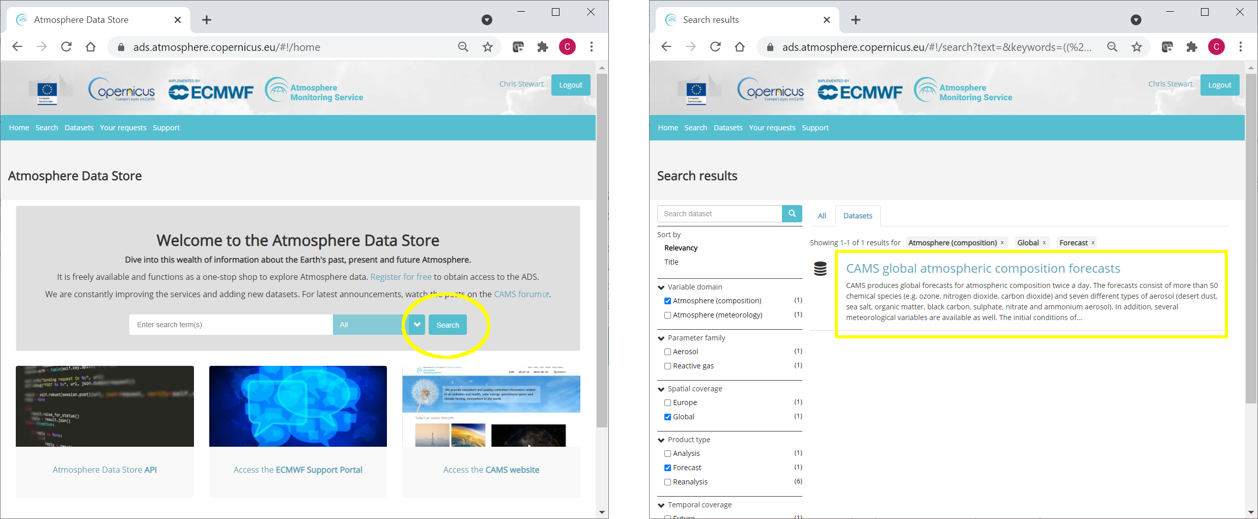
Having selected the correct dataset, we now need to specify what product type, variables, temporal and geographic coverage we are interested in. These can all be selected in the Download data tab, where a form appears in which we will select the following parameters to download:

• Variables (Single level): Dust aerosol optical depth at 550nm, Organic matter aerosol optical depth at 550nm, Total aerosol optical depth at 550nm

• Date: Start: 2021-08-01, End: 2021-08-08

• Time: 00:00, 12:00 (default)

• Leadtime hour: 0 (only analysis)

• Type: Forecast (default)

• Area: Restricted area: North: 90, East: 180, South: 0, West: -180

• Format: Zipped netCDF (experimental)

At the end of the download form, select Show API request. This will reveal a block of that you can copy and paste into a cell of your Jupyter Notebook, like this:

c = cdsapi.Client(url=URL, key=KEY)
c.retrieve(
    'cams-global-atmospheric-composition-forecasts',
    {
        'variable': [
            'dust_aerosol_optical_depth_550nm', 'organic_matter_aerosol_optical_depth_550nm', 'total_aerosol_optical_depth_550nm',
        ],
        'date': '2021-08-01/2021-08-08',
        'time': [
            '00:00', '12:00',
        ],
        'leadtime_hour': '0',
        'type': 'forecast',
        'area': [
            90, -180, 0,
            180,
        ],
        'format': 'netcdf_zip',
    },
    f'{DATADIR}/2021-08_AOD.zip')

2024-06-06 11:54:39,748 INFO Welcome to the CDS
2024-06-06 11:54:39,750 INFO Sending request to https://ads.atmosphere.copernicus.eu/api/v2/resources/cams-global-atmospheric-composition-forecasts
2024-06-06 11:54:39,905 INFO Request is completed
2024-06-06 11:54:39,907 INFO Downloading https://download-0003-ads-clone.copernicus-climate.eu/cache-compute-0003/cache/data8/adaptor.mars_constrained.external-1713606098.3237348-20916-11-e864f29f-79e5-455c-911d-cb25cc6e8fd6.zip to .//2021-08_AOD.zip (18.6M)
2024-06-06 11:54:43,670 INFO Download rate 5M/s                                 

Result(content_length=19532732,content_type=application/zip,location=https://download-0003-ads-clone.copernicus-climate.eu/cache-compute-0003/cache/data8/adaptor.mars_constrained.external-1713606098.3237348-20916-11-e864f29f-79e5-455c-911d-cb25cc6e8fd6.zip)

---

3. Read data with the xarray library

We have requested the data in NetCDF format. This is a commonly used format for gridded (array-based) scientific data, which is data that has the following characteristics:

• A regular, evenly spaced grid structure where each point on the grid is defined by its coordinates (e.g., latitude, longitude, altitude, or time) and has a corresponding value for a variable (e.g., temperature).

• One or multiple dimensions, which is why they are referred to as multidimensional or ND arrays. Examples of dimensions can be:

  • 1D: time series (as temperature over time at a single location).

  • 2D: Spatial data (as sea surface temperature over an area).

  • 3D: Volumetric data (as atmospheric temperature at various altitudes).

  • 4D: spatiotemporal data (as temperature over an area at different times).

To read and process this data we will make use of the Xarray library. Xarray is an open source project and Python package that makes working with labelled multi-dimensional arrays simple and efficient.

We will read the data from our NetCDF file into an Xarray dataset. For this, first we extract the downloaded zip file:

# Create a ZipFile Object and load zip file in it
with ZipFile(f'{DATADIR}/2021-08_AOD.zip', 'r') as zipObj:
   # Extract all the contents of zip file into a directory
   zipObj.extractall(path=f'{DATADIR}/2021-08_AOD/')

For convenience, we create a variable with the name of our downloaded file:

fn = f'{DATADIR}/2021-08_AOD/data.nc'

Now we can read the data into an Xarray dataset:

# Create Xarray Dataset
ds = xr.open_dataset(fn)

And see how it looks like:

ds

<xarray.Dataset> Size: 78MB
Dimensions:    (longitude: 900, latitude: 226, time: 16)
Coordinates:
  * longitude  (longitude) float32 4kB -180.0 -179.6 -179.2 ... 179.2 179.6
  * latitude   (latitude) float32 904B 90.0 89.6 89.2 88.8 ... 1.2 0.8 0.4 0.0
  * time       (time) datetime64[ns] 128B 2021-08-01 ... 2021-08-08T12:00:00
Data variables:
    omaod550   (time, latitude, longitude) float64 26MB ...
    aod550     (time, latitude, longitude) float64 26MB ...
    duaod550   (time, latitude, longitude) float64 26MB ...
Attributes:
    Conventions:  CF-1.6
    history:      2024-04-20 09:41:37 GMT by grib_to_netcdf-2.25.1: /opt/ecmw...

xarray.Dataset

• Dimensions:
  • longitude: 900
  • latitude: 226
  • time: 16
• Coordinates: (3)
  • longitude
    (longitude)
    float32
    -180.0 -179.6 ... 179.2 179.6

    units :

    degrees_east

    long_name :

    longitude

    array([-180. , -179.6, -179.2, ...,  178.8,  179.2,  179.6], dtype=float32)

  • latitude
    (latitude)
    float32
    90.0 89.6 89.2 88.8 ... 0.8 0.4 0.0

    units :

    degrees_north

    long_name :

    latitude

    array([90. , 89.6, 89.2, ...,  0.8,  0.4,  0. ], dtype=float32)

  • time
    (time)
    datetime64[ns]
    2021-08-01 ... 2021-08-08T12:00:00

    long_name :

    time

    array(['2021-08-01T00:00:00.000000000', '2021-08-01T12:00:00.000000000',
           '2021-08-02T00:00:00.000000000', '2021-08-02T12:00:00.000000000',
           '2021-08-03T00:00:00.000000000', '2021-08-03T12:00:00.000000000',
           '2021-08-04T00:00:00.000000000', '2021-08-04T12:00:00.000000000',
           '2021-08-05T00:00:00.000000000', '2021-08-05T12:00:00.000000000',
           '2021-08-06T00:00:00.000000000', '2021-08-06T12:00:00.000000000',
           '2021-08-07T00:00:00.000000000', '2021-08-07T12:00:00.000000000',
           '2021-08-08T00:00:00.000000000', '2021-08-08T12:00:00.000000000'],
          dtype='datetime64[ns]')

• Data variables: (3)
  • omaod550
    (time, latitude, longitude)
    float64
    ...

    units :

    ~

    long_name :

    Organic Matter Aerosol Optical Depth at 550nm

    [3254400 values with dtype=float64]

  • aod550
    (time, latitude, longitude)
    float64
    ...

    units :

    ~

    long_name :

    Total Aerosol Optical Depth at 550nm

    [3254400 values with dtype=float64]

  • duaod550
    (time, latitude, longitude)
    float64
    ...

    units :

    ~

    long_name :

    Dust Aerosol Optical Depth at 550nm

    [3254400 values with dtype=float64]

• Indexes: (3)
  • longitude
    PandasIndex

    PandasIndex(Index([             -180.0, -179.60000610351562,  -179.1999969482422,
            -178.8000030517578, -178.39999389648438,              -178.0,
           -177.60000610351562,  -177.1999969482422,  -176.8000030517578,
           -176.39999389648438,
           ...
                         176.0,  176.39999389648438,   176.8000030517578,
             177.1999969482422,  177.60000610351562,               178.0,
            178.39999389648438,   178.8000030517578,   179.1999969482422,
            179.60000610351562],
          dtype='float32', name='longitude', length=900))

  • latitude
    PandasIndex

    PandasIndex(Index([              90.0,   89.5999984741211,  89.19999694824219,
            88.80000305175781,   88.4000015258789,               88.0,
             87.5999984741211,  87.19999694824219,  86.80000305175781,
             86.4000015258789,
           ...
           3.5999999046325684,  3.200000047683716,  2.799999952316284,
           2.4000000953674316,                2.0,  1.600000023841858,
           1.2000000476837158,  0.800000011920929, 0.4000000059604645,
                          0.0],
          dtype='float32', name='latitude', length=226))

  • time
    PandasIndex

    PandasIndex(DatetimeIndex(['2021-08-01 00:00:00', '2021-08-01 12:00:00',
                   '2021-08-02 00:00:00', '2021-08-02 12:00:00',
                   '2021-08-03 00:00:00', '2021-08-03 12:00:00',
                   '2021-08-04 00:00:00', '2021-08-04 12:00:00',
                   '2021-08-05 00:00:00', '2021-08-05 12:00:00',
                   '2021-08-06 00:00:00', '2021-08-06 12:00:00',
                   '2021-08-07 00:00:00', '2021-08-07 12:00:00',
                   '2021-08-08 00:00:00', '2021-08-08 12:00:00'],
                  dtype='datetime64[ns]', name='time', freq=None))

• Attributes: (2)

  Conventions :

  CF-1.6

  history :

  2024-04-20 09:41:37 GMT by grib_to_netcdf-2.25.1: /opt/ecmwf/mars-client/bin/grib_to_netcdf.bin -S param -o /cache/tmp/e864f29f-79e5-455c-911d-cb25cc6e8fd6-adaptor.mars_constrained.external-1713606097.5984967-20916-24-tmp.nc /cache/tmp/e864f29f-79e5-455c-911d-cb25cc6e8fd6-adaptor.mars_constrained.external-1713606097.489146-20916-23-tmp.grib

We see that the dataset has three variables. Selecting the show/hide attributes icons reveals their names:

• omaod550 is Organic Matter Aerosol Optical Depth at 550nm

• aod550 is Total Aerosol Optical Depth at 550nm and

• duaod550 is Dust Aerosol Optical Depth at 550nm

The dataset also has three dimensions: longitude, latitude and time.

We will now look more carefully at the Total Aerosol Optical Depth at 550nm dataset.

While an Xarray dataset may contain multiple variables, an Xarray data array holds a single multi-dimensional variable and its coordinates. To make the processing of the aod550 data easier, we convert in into an Xarray data array.

# Create Xarray Data Array
da = ds['aod550']
da

<xarray.DataArray 'aod550' (time: 16, latitude: 226, longitude: 900)> Size: 26MB
[3254400 values with dtype=float64]
Coordinates:
  * longitude  (longitude) float32 4kB -180.0 -179.6 -179.2 ... 179.2 179.6
  * latitude   (latitude) float32 904B 90.0 89.6 89.2 88.8 ... 1.2 0.8 0.4 0.0
  * time       (time) datetime64[ns] 128B 2021-08-01 ... 2021-08-08T12:00:00
Attributes:
    units:      ~
    long_name:  Total Aerosol Optical Depth at 550nm

xarray.DataArray

'aod550'

• time: 16
• latitude: 226
• longitude: 900

• ...

  [3254400 values with dtype=float64]

• Coordinates: (3)
  • longitude
    (longitude)
    float32
    -180.0 -179.6 ... 179.2 179.6

    units :

    degrees_east

    long_name :

    longitude

    array([-180. , -179.6, -179.2, ...,  178.8,  179.2,  179.6], dtype=float32)

  • latitude
    (latitude)
    float32
    90.0 89.6 89.2 88.8 ... 0.8 0.4 0.0

    units :

    degrees_north

    long_name :

    latitude

    array([90. , 89.6, 89.2, ...,  0.8,  0.4,  0. ], dtype=float32)

  • time
    (time)
    datetime64[ns]
    2021-08-01 ... 2021-08-08T12:00:00

    long_name :

    time

    array(['2021-08-01T00:00:00.000000000', '2021-08-01T12:00:00.000000000',
           '2021-08-02T00:00:00.000000000', '2021-08-02T12:00:00.000000000',
           '2021-08-03T00:00:00.000000000', '2021-08-03T12:00:00.000000000',
           '2021-08-04T00:00:00.000000000', '2021-08-04T12:00:00.000000000',
           '2021-08-05T00:00:00.000000000', '2021-08-05T12:00:00.000000000',
           '2021-08-06T00:00:00.000000000', '2021-08-06T12:00:00.000000000',
           '2021-08-07T00:00:00.000000000', '2021-08-07T12:00:00.000000000',
           '2021-08-08T00:00:00.000000000', '2021-08-08T12:00:00.000000000'],
          dtype='datetime64[ns]')

• Indexes: (3)
  • longitude
    PandasIndex

    PandasIndex(Index([             -180.0, -179.60000610351562,  -179.1999969482422,
            -178.8000030517578, -178.39999389648438,              -178.0,
           -177.60000610351562,  -177.1999969482422,  -176.8000030517578,
           -176.39999389648438,
           ...
                         176.0,  176.39999389648438,   176.8000030517578,
             177.1999969482422,  177.60000610351562,               178.0,
            178.39999389648438,   178.8000030517578,   179.1999969482422,
            179.60000610351562],
          dtype='float32', name='longitude', length=900))

  • latitude
    PandasIndex

    PandasIndex(Index([              90.0,   89.5999984741211,  89.19999694824219,
            88.80000305175781,   88.4000015258789,               88.0,
             87.5999984741211,  87.19999694824219,  86.80000305175781,
             86.4000015258789,
           ...
           3.5999999046325684,  3.200000047683716,  2.799999952316284,
           2.4000000953674316,                2.0,  1.600000023841858,
           1.2000000476837158,  0.800000011920929, 0.4000000059604645,
                          0.0],
          dtype='float32', name='latitude', length=226))

  • time
    PandasIndex

    PandasIndex(DatetimeIndex(['2021-08-01 00:00:00', '2021-08-01 12:00:00',
                   '2021-08-02 00:00:00', '2021-08-02 12:00:00',
                   '2021-08-03 00:00:00', '2021-08-03 12:00:00',
                   '2021-08-04 00:00:00', '2021-08-04 12:00:00',
                   '2021-08-05 00:00:00', '2021-08-05 12:00:00',
                   '2021-08-06 00:00:00', '2021-08-06 12:00:00',
                   '2021-08-07 00:00:00', '2021-08-07 12:00:00',
                   '2021-08-08 00:00:00', '2021-08-08 12:00:00'],
                  dtype='datetime64[ns]', name='time', freq=None))

• Attributes: (2)

  units :

  ~

  long_name :

  Total Aerosol Optical Depth at 550nm

---

4. Subset data

This section provides some selected examples of ways in which parts of a dataset can be extracted. More comprehensive documentation on how to index and select data is available here.

---

4.A. Temporal subset

By inspecting the array, we notice that the first of the three dimensions is time (see first line of the output above). If we wish to select only one time step, the easiest way to do this is to use positional indexing. The code below creates a Data Array of only the first time step.

time0 = da[0,:,:]
time0

<xarray.DataArray 'aod550' (latitude: 226, longitude: 900)> Size: 2MB
[203400 values with dtype=float64]
Coordinates:
  * longitude  (longitude) float32 4kB -180.0 -179.6 -179.2 ... 179.2 179.6
  * latitude   (latitude) float32 904B 90.0 89.6 89.2 88.8 ... 1.2 0.8 0.4 0.0
    time       datetime64[ns] 8B 2021-08-01
Attributes:
    units:      ~
    long_name:  Total Aerosol Optical Depth at 550nm

xarray.DataArray

'aod550'

• latitude: 226
• longitude: 900

• ...

  [203400 values with dtype=float64]

• Coordinates: (3)
  • longitude
    (longitude)
    float32
    -180.0 -179.6 ... 179.2 179.6

    units :

    degrees_east

    long_name :

    longitude

    array([-180. , -179.6, -179.2, ...,  178.8,  179.2,  179.6], dtype=float32)

  • latitude
    (latitude)
    float32
    90.0 89.6 89.2 88.8 ... 0.8 0.4 0.0

    units :

    degrees_north

    long_name :

    latitude

    array([90. , 89.6, 89.2, ...,  0.8,  0.4,  0. ], dtype=float32)

  • time
    ()
    datetime64[ns]
    2021-08-01

    long_name :

    time

    array('2021-08-01T00:00:00.000000000', dtype='datetime64[ns]')

• Indexes: (2)
  • longitude
    PandasIndex

    PandasIndex(Index([             -180.0, -179.60000610351562,  -179.1999969482422,
            -178.8000030517578, -178.39999389648438,              -178.0,
           -177.60000610351562,  -177.1999969482422,  -176.8000030517578,
           -176.39999389648438,
           ...
                         176.0,  176.39999389648438,   176.8000030517578,
             177.1999969482422,  177.60000610351562,               178.0,
            178.39999389648438,   178.8000030517578,   179.1999969482422,
            179.60000610351562],
          dtype='float32', name='longitude', length=900))

  • latitude
    PandasIndex

    PandasIndex(Index([              90.0,   89.5999984741211,  89.19999694824219,
            88.80000305175781,   88.4000015258789,               88.0,
             87.5999984741211,  87.19999694824219,  86.80000305175781,
             86.4000015258789,
           ...
           3.5999999046325684,  3.200000047683716,  2.799999952316284,
           2.4000000953674316,                2.0,  1.600000023841858,
           1.2000000476837158,  0.800000011920929, 0.4000000059604645,
                          0.0],
          dtype='float32', name='latitude', length=226))

• Attributes: (2)

  units :

  ~

  long_name :

  Total Aerosol Optical Depth at 550nm

And this creates a Data Array of the first 5 time steps:

time_5steps = da[0:5,:,:]
time_5steps

<xarray.DataArray 'aod550' (time: 5, latitude: 226, longitude: 900)> Size: 8MB
[1017000 values with dtype=float64]
Coordinates:
  * longitude  (longitude) float32 4kB -180.0 -179.6 -179.2 ... 179.2 179.6
  * latitude   (latitude) float32 904B 90.0 89.6 89.2 88.8 ... 1.2 0.8 0.4 0.0
  * time       (time) datetime64[ns] 40B 2021-08-01 ... 2021-08-03
Attributes:
    units:      ~
    long_name:  Total Aerosol Optical Depth at 550nm

xarray.DataArray

'aod550'

• time: 5
• latitude: 226
• longitude: 900

• ...

  [1017000 values with dtype=float64]

• Coordinates: (3)
  • longitude
    (longitude)
    float32
    -180.0 -179.6 ... 179.2 179.6

    units :

    degrees_east

    long_name :

    longitude

    array([-180. , -179.6, -179.2, ...,  178.8,  179.2,  179.6], dtype=float32)

  • latitude
    (latitude)
    float32
    90.0 89.6 89.2 88.8 ... 0.8 0.4 0.0

    units :

    degrees_north

    long_name :

    latitude

    array([90. , 89.6, 89.2, ...,  0.8,  0.4,  0. ], dtype=float32)

  • time
    (time)
    datetime64[ns]
    2021-08-01 ... 2021-08-03

    long_name :

    time

    array(['2021-08-01T00:00:00.000000000', '2021-08-01T12:00:00.000000000',
           '2021-08-02T00:00:00.000000000', '2021-08-02T12:00:00.000000000',
           '2021-08-03T00:00:00.000000000'], dtype='datetime64[ns]')

• Indexes: (3)
  • longitude
    PandasIndex

    PandasIndex(Index([             -180.0, -179.60000610351562,  -179.1999969482422,
            -178.8000030517578, -178.39999389648438,              -178.0,
           -177.60000610351562,  -177.1999969482422,  -176.8000030517578,
           -176.39999389648438,
           ...
                         176.0,  176.39999389648438,   176.8000030517578,
             177.1999969482422,  177.60000610351562,               178.0,
            178.39999389648438,   178.8000030517578,   179.1999969482422,
            179.60000610351562],
          dtype='float32', name='longitude', length=900))

  • latitude
    PandasIndex

    PandasIndex(Index([              90.0,   89.5999984741211,  89.19999694824219,
            88.80000305175781,   88.4000015258789,               88.0,
             87.5999984741211,  87.19999694824219,  86.80000305175781,
             86.4000015258789,
           ...
           3.5999999046325684,  3.200000047683716,  2.799999952316284,
           2.4000000953674316,                2.0,  1.600000023841858,
           1.2000000476837158,  0.800000011920929, 0.4000000059604645,
                          0.0],
          dtype='float32', name='latitude', length=226))

  • time
    PandasIndex

    PandasIndex(DatetimeIndex(['2021-08-01 00:00:00', '2021-08-01 12:00:00',
                   '2021-08-02 00:00:00', '2021-08-02 12:00:00',
                   '2021-08-03 00:00:00'],
                  dtype='datetime64[ns]', name='time', freq=None))

• Attributes: (2)

  units :

  ~

  long_name :

  Total Aerosol Optical Depth at 550nm

Another way to select data is to use the .sel() method of xarray. The example below selects all data from the first of August.

firstAug = da.sel(time='2021-08-01')

We can also select a time range using label based indexing, with the loc attribute:

period = da.loc["2021-08-01":"2021-08-03"]
period

<xarray.DataArray 'aod550' (time: 6, latitude: 226, longitude: 900)> Size: 10MB
[1220400 values with dtype=float64]
Coordinates:
  * longitude  (longitude) float32 4kB -180.0 -179.6 -179.2 ... 179.2 179.6
  * latitude   (latitude) float32 904B 90.0 89.6 89.2 88.8 ... 1.2 0.8 0.4 0.0
  * time       (time) datetime64[ns] 48B 2021-08-01 ... 2021-08-03T12:00:00
Attributes:
    units:      ~
    long_name:  Total Aerosol Optical Depth at 550nm

xarray.DataArray

'aod550'

• time: 6
• latitude: 226
• longitude: 900

• ...

  [1220400 values with dtype=float64]

• Coordinates: (3)
  • longitude
    (longitude)
    float32
    -180.0 -179.6 ... 179.2 179.6

    units :

    degrees_east

    long_name :

    longitude

    array([-180. , -179.6, -179.2, ...,  178.8,  179.2,  179.6], dtype=float32)

  • latitude
    (latitude)
    float32
    90.0 89.6 89.2 88.8 ... 0.8 0.4 0.0

    units :

    degrees_north

    long_name :

    latitude

    array([90. , 89.6, 89.2, ...,  0.8,  0.4,  0. ], dtype=float32)

  • time
    (time)
    datetime64[ns]
    2021-08-01 ... 2021-08-03T12:00:00

    long_name :

    time

    array(['2021-08-01T00:00:00.000000000', '2021-08-01T12:00:00.000000000',
           '2021-08-02T00:00:00.000000000', '2021-08-02T12:00:00.000000000',
           '2021-08-03T00:00:00.000000000', '2021-08-03T12:00:00.000000000'],
          dtype='datetime64[ns]')

• Indexes: (3)
  • longitude
    PandasIndex

    PandasIndex(Index([             -180.0, -179.60000610351562,  -179.1999969482422,
            -178.8000030517578, -178.39999389648438,              -178.0,
           -177.60000610351562,  -177.1999969482422,  -176.8000030517578,
           -176.39999389648438,
           ...
                         176.0,  176.39999389648438,   176.8000030517578,
             177.1999969482422,  177.60000610351562,               178.0,
            178.39999389648438,   178.8000030517578,   179.1999969482422,
            179.60000610351562],
          dtype='float32', name='longitude', length=900))

  • latitude
    PandasIndex

    PandasIndex(Index([              90.0,   89.5999984741211,  89.19999694824219,
            88.80000305175781,   88.4000015258789,               88.0,
             87.5999984741211,  87.19999694824219,  86.80000305175781,
             86.4000015258789,
           ...
           3.5999999046325684,  3.200000047683716,  2.799999952316284,
           2.4000000953674316,                2.0,  1.600000023841858,
           1.2000000476837158,  0.800000011920929, 0.4000000059604645,
                          0.0],
          dtype='float32', name='latitude', length=226))

  • time
    PandasIndex

    PandasIndex(DatetimeIndex(['2021-08-01 00:00:00', '2021-08-01 12:00:00',
                   '2021-08-02 00:00:00', '2021-08-02 12:00:00',
                   '2021-08-03 00:00:00', '2021-08-03 12:00:00'],
                  dtype='datetime64[ns]', name='time', freq=None))

• Attributes: (2)

  units :

  ~

  long_name :

  Total Aerosol Optical Depth at 550nm

---

4.B. Geographic subset

Geographical subsetting works in much the same way as temporal subsetting, with the difference that instead of one dimension we now have two (or even three if we include altitude).

Select nearest grid cell

In some cases, we may want to find the geographic grid cell that is situated nearest to a particular location of interest, such as a city. In this case we can use .sel(), and make use of the method keyword argument, which enables nearest neighbor (inexact) lookups. In the example below, we look for the geographic grid cell nearest to Paris.

paris_lat = 48.9
paris_lon = 2.4

paris = da.sel(latitude=paris_lat, longitude=paris_lon, method='nearest')

paris

<xarray.DataArray 'aod550' (time: 16)> Size: 128B
[16 values with dtype=float64]
Coordinates:
    longitude  float32 4B 2.4
    latitude   float32 4B 48.8
  * time       (time) datetime64[ns] 128B 2021-08-01 ... 2021-08-08T12:00:00
Attributes:
    units:      ~
    long_name:  Total Aerosol Optical Depth at 550nm

xarray.DataArray

'aod550'

• time: 16

• ...

  [16 values with dtype=float64]

• Coordinates: (3)
  • longitude
    ()
    float32
    2.4

    units :

    degrees_east

    long_name :

    longitude

    array(2.4, dtype=float32)

  • latitude
    ()
    float32
    48.8

    units :

    degrees_north

    long_name :

    latitude

    array(48.8, dtype=float32)

  • time
    (time)
    datetime64[ns]
    2021-08-01 ... 2021-08-08T12:00:00

    long_name :

    time

    array(['2021-08-01T00:00:00.000000000', '2021-08-01T12:00:00.000000000',
           '2021-08-02T00:00:00.000000000', '2021-08-02T12:00:00.000000000',
           '2021-08-03T00:00:00.000000000', '2021-08-03T12:00:00.000000000',
           '2021-08-04T00:00:00.000000000', '2021-08-04T12:00:00.000000000',
           '2021-08-05T00:00:00.000000000', '2021-08-05T12:00:00.000000000',
           '2021-08-06T00:00:00.000000000', '2021-08-06T12:00:00.000000000',
           '2021-08-07T00:00:00.000000000', '2021-08-07T12:00:00.000000000',
           '2021-08-08T00:00:00.000000000', '2021-08-08T12:00:00.000000000'],
          dtype='datetime64[ns]')

• Indexes: (1)
  • time
    PandasIndex

    PandasIndex(DatetimeIndex(['2021-08-01 00:00:00', '2021-08-01 12:00:00',
                   '2021-08-02 00:00:00', '2021-08-02 12:00:00',
                   '2021-08-03 00:00:00', '2021-08-03 12:00:00',
                   '2021-08-04 00:00:00', '2021-08-04 12:00:00',
                   '2021-08-05 00:00:00', '2021-08-05 12:00:00',
                   '2021-08-06 00:00:00', '2021-08-06 12:00:00',
                   '2021-08-07 00:00:00', '2021-08-07 12:00:00',
                   '2021-08-08 00:00:00', '2021-08-08 12:00:00'],
                  dtype='datetime64[ns]', name='time', freq=None))

• Attributes: (2)

  units :

  ~

  long_name :

  Total Aerosol Optical Depth at 550nm

Regional subset

Often we may wish to select a regional subset. Note that you can specify a region of interest in the ADS prior to downloading data. This is more efficient as it reduces the data volume. However, there may be cases when you wish to select a regional subset after download. One way to do this is with the .where() function.

In the previous examples, we have used methods that return a subset of the original data. By default .where() maintains the original size of the data and masks unselected elements (which become “not a number”, or nan). By using the option drop=True you can then clip the elements that are masked.

The example below uses .where() to select a geographic subset from 30 to 60 degrees latitude. We could also specify longitudinal boundaries by simply adding further conditions.

mid_lat = da.where((da.latitude > 30.) & (da.latitude < 60.), drop=True)

---

5. Aggregate data

Another common task is to aggregate data. This may include reducing hourly data to daily means, minimum, maximum, or other statistical properties. We may wish to apply the aggregation over one or more dimensions, such as averaging over all latitudes and longitudes to obtain one global value.

---

5.A. Temporal aggregation

To aggregate over one or more dimensions, we can apply one of a number of methods to the original dataset, such as .mean(), .min(), .max(), .median() and others (see full list here).

The example below takes the mean of all time steps. The keep_attrs parameter is optional. If set to True it will keep the original attributes of the Data Array (i.e. description of variable, units, etc). If set to false, the attributes will be stripped.

time_mean = da.mean(dim="time", keep_attrs=True)
time_mean

<xarray.DataArray 'aod550' (latitude: 226, longitude: 900)> Size: 2MB
array([[0.50736934, 0.50736934, 0.50736934, ..., 0.50736934, 0.50736934,
        0.50736934],
       [0.46712606, 0.46684634, 0.4665423 , ..., 0.46802603, 0.46777064,
        0.46744227],
       [0.43602844, 0.43542035, 0.43483658, ..., 0.43786486, 0.43722029,
        0.43663652],
       ...,
       [0.07073772, 0.06998369, 0.06994721, ..., 0.07223362, 0.07047016,
        0.070458  ],
       [0.07082285, 0.06885265, 0.06729594, ..., 0.07398491, 0.07276873,
        0.07190525],
       [0.06977694, 0.06662704, 0.06412172, ..., 0.07569972, 0.07466597,
        0.07248901]])
Coordinates:
  * longitude  (longitude) float32 4kB -180.0 -179.6 -179.2 ... 179.2 179.6
  * latitude   (latitude) float32 904B 90.0 89.6 89.2 88.8 ... 1.2 0.8 0.4 0.0
Attributes:
    units:      ~
    long_name:  Total Aerosol Optical Depth at 550nm

xarray.DataArray

'aod550'

• latitude: 226
• longitude: 900

• 0.5074 0.5074 0.5074 0.5074 0.5074 ... 0.07807 0.0757 0.07467 0.07249

  array([[0.50736934, 0.50736934, 0.50736934, ..., 0.50736934, 0.50736934,
          0.50736934],
         [0.46712606, 0.46684634, 0.4665423 , ..., 0.46802603, 0.46777064,
          0.46744227],
         [0.43602844, 0.43542035, 0.43483658, ..., 0.43786486, 0.43722029,
          0.43663652],
         ...,
         [0.07073772, 0.06998369, 0.06994721, ..., 0.07223362, 0.07047016,
          0.070458  ],
         [0.07082285, 0.06885265, 0.06729594, ..., 0.07398491, 0.07276873,
          0.07190525],
         [0.06977694, 0.06662704, 0.06412172, ..., 0.07569972, 0.07466597,
          0.07248901]])

• Coordinates: (2)
  • longitude
    (longitude)
    float32
    -180.0 -179.6 ... 179.2 179.6

    units :

    degrees_east

    long_name :

    longitude

    array([-180. , -179.6, -179.2, ...,  178.8,  179.2,  179.6], dtype=float32)

  • latitude
    (latitude)
    float32
    90.0 89.6 89.2 88.8 ... 0.8 0.4 0.0

    units :

    degrees_north

    long_name :

    latitude

    array([90. , 89.6, 89.2, ...,  0.8,  0.4,  0. ], dtype=float32)

• Indexes: (2)
  • longitude
    PandasIndex

    PandasIndex(Index([             -180.0, -179.60000610351562,  -179.1999969482422,
            -178.8000030517578, -178.39999389648438,              -178.0,
           -177.60000610351562,  -177.1999969482422,  -176.8000030517578,
           -176.39999389648438,
           ...
                         176.0,  176.39999389648438,   176.8000030517578,
             177.1999969482422,  177.60000610351562,               178.0,
            178.39999389648438,   178.8000030517578,   179.1999969482422,
            179.60000610351562],
          dtype='float32', name='longitude', length=900))

  • latitude
    PandasIndex

    PandasIndex(Index([              90.0,   89.5999984741211,  89.19999694824219,
            88.80000305175781,   88.4000015258789,               88.0,
             87.5999984741211,  87.19999694824219,  86.80000305175781,
             86.4000015258789,
           ...
           3.5999999046325684,  3.200000047683716,  2.799999952316284,
           2.4000000953674316,                2.0,  1.600000023841858,
           1.2000000476837158,  0.800000011920929, 0.4000000059604645,
                          0.0],
          dtype='float32', name='latitude', length=226))

• Attributes: (2)

  units :

  ~

  long_name :

  Total Aerosol Optical Depth at 550nm

Instead of reducing an entire dimension to one value, we may wish to reduce the frequency within a dimension. For example, we can reduce hourly data to daily max values. One way to do this is using groupby() combined with the .max() aggregate function, as shown below:

daily_max = da.groupby('time.day').max(keep_attrs=True)
daily_max

<xarray.DataArray 'aod550' (day: 8, latitude: 226, longitude: 900)> Size: 13MB
array([[[0.2626625 , 0.2626625 , 0.2626625 , ..., 0.2626625 ,
         0.2626625 , 0.2626625 ],
        [0.22588533, 0.22530157, 0.2247178 , ..., 0.22783121,
         0.22724745, 0.22666368],
        [0.24534415, 0.24417662, 0.24281451, ..., 0.24923592,
         0.24806839, 0.24670627],
        ...,
        [0.09843005, 0.09473288, 0.08714394, ..., 0.10348935,
         0.10076511, 0.09862464],
        [0.12431029, 0.11516464, 0.10057052, ..., 0.11613758,
         0.11146746, 0.1190564 ],
        [0.11788888, 0.11788888, 0.10854864, ..., 0.11886182,
         0.11555382, 0.11633217]],

       [[2.56833819, 2.56833819, 2.56833819, ..., 2.56833819,
         2.56833819, 2.56833819],
        [2.66037842, 2.65979465, 2.65921089, ..., 2.66193512,
         2.66135136, 2.66076759],
        [2.51424267, 2.51326973, 2.51229679, ..., 2.51755067,
         2.51638314, 2.5154102 ],
...
        [0.09570582, 0.09531664, 0.09414911, ..., 0.08733853,
         0.09200864, 0.09375994],
        [0.099403  , 0.09843005, 0.09570582, ..., 0.08811688,
         0.092787  , 0.09570582],
        [0.09628958, 0.0943437 , 0.092787  , ..., 0.0877277 ,
         0.09259241, 0.09473288]],

       [[0.09901382, 0.09901382, 0.09901382, ..., 0.09901382,
         0.09901382, 0.09901382],
        [0.10348935, 0.10348935, 0.10329476, ..., 0.10387852,
         0.10387852, 0.10368394],
        [0.11282958, 0.11263499, 0.11244041, ..., 0.11341335,
         0.11321876, 0.11302417],
        ...,
        [0.06359876, 0.07605241, 0.08208464, ..., 0.06087453,
         0.05776112, 0.05756653],
        [0.05523147, 0.06106912, 0.06204206, ..., 0.06282041,
         0.05795571, 0.05503688],
        [0.05445312, 0.05250724, 0.0482263 , ..., 0.07060394,
         0.06573924, 0.05951241]]])
Coordinates:
  * longitude  (longitude) float32 4kB -180.0 -179.6 -179.2 ... 179.2 179.6
  * latitude   (latitude) float32 904B 90.0 89.6 89.2 88.8 ... 1.2 0.8 0.4 0.0
  * day        (day) int64 64B 1 2 3 4 5 6 7 8
Attributes:
    units:      ~
    long_name:  Total Aerosol Optical Depth at 550nm

xarray.DataArray

'aod550'

• day: 8
• latitude: 226
• longitude: 900

• 0.2627 0.2627 0.2627 0.2627 0.2627 ... 0.0706 0.0706 0.06574 0.05951

  array([[[0.2626625 , 0.2626625 , 0.2626625 , ..., 0.2626625 ,
           0.2626625 , 0.2626625 ],
          [0.22588533, 0.22530157, 0.2247178 , ..., 0.22783121,
           0.22724745, 0.22666368],
          [0.24534415, 0.24417662, 0.24281451, ..., 0.24923592,
           0.24806839, 0.24670627],
          ...,
          [0.09843005, 0.09473288, 0.08714394, ..., 0.10348935,
           0.10076511, 0.09862464],
          [0.12431029, 0.11516464, 0.10057052, ..., 0.11613758,
           0.11146746, 0.1190564 ],
          [0.11788888, 0.11788888, 0.10854864, ..., 0.11886182,
           0.11555382, 0.11633217]],
  
         [[2.56833819, 2.56833819, 2.56833819, ..., 2.56833819,
           2.56833819, 2.56833819],
          [2.66037842, 2.65979465, 2.65921089, ..., 2.66193512,
           2.66135136, 2.66076759],
          [2.51424267, 2.51326973, 2.51229679, ..., 2.51755067,
           2.51638314, 2.5154102 ],
  ...
          [0.09570582, 0.09531664, 0.09414911, ..., 0.08733853,
           0.09200864, 0.09375994],
          [0.099403  , 0.09843005, 0.09570582, ..., 0.08811688,
           0.092787  , 0.09570582],
          [0.09628958, 0.0943437 , 0.092787  , ..., 0.0877277 ,
           0.09259241, 0.09473288]],
  
         [[0.09901382, 0.09901382, 0.09901382, ..., 0.09901382,
           0.09901382, 0.09901382],
          [0.10348935, 0.10348935, 0.10329476, ..., 0.10387852,
           0.10387852, 0.10368394],
          [0.11282958, 0.11263499, 0.11244041, ..., 0.11341335,
           0.11321876, 0.11302417],
          ...,
          [0.06359876, 0.07605241, 0.08208464, ..., 0.06087453,
           0.05776112, 0.05756653],
          [0.05523147, 0.06106912, 0.06204206, ..., 0.06282041,
           0.05795571, 0.05503688],
          [0.05445312, 0.05250724, 0.0482263 , ..., 0.07060394,
           0.06573924, 0.05951241]]])

• Coordinates: (3)
  • longitude
    (longitude)
    float32
    -180.0 -179.6 ... 179.2 179.6

    units :

    degrees_east

    long_name :

    longitude

    array([-180. , -179.6, -179.2, ...,  178.8,  179.2,  179.6], dtype=float32)

  • latitude
    (latitude)
    float32
    90.0 89.6 89.2 88.8 ... 0.8 0.4 0.0

    units :

    degrees_north

    long_name :

    latitude

    array([90. , 89.6, 89.2, ...,  0.8,  0.4,  0. ], dtype=float32)

  • day
    (day)
    int64
    1 2 3 4 5 6 7 8

    array([1, 2, 3, 4, 5, 6, 7, 8])

• Indexes: (3)
  • longitude
    PandasIndex

    PandasIndex(Index([             -180.0, -179.60000610351562,  -179.1999969482422,
            -178.8000030517578, -178.39999389648438,              -178.0,
           -177.60000610351562,  -177.1999969482422,  -176.8000030517578,
           -176.39999389648438,
           ...
                         176.0,  176.39999389648438,   176.8000030517578,
             177.1999969482422,  177.60000610351562,               178.0,
            178.39999389648438,   178.8000030517578,   179.1999969482422,
            179.60000610351562],
          dtype='float32', name='longitude', length=900))

  • latitude
    PandasIndex

    PandasIndex(Index([              90.0,   89.5999984741211,  89.19999694824219,
            88.80000305175781,   88.4000015258789,               88.0,
             87.5999984741211,  87.19999694824219,  86.80000305175781,
             86.4000015258789,
           ...
           3.5999999046325684,  3.200000047683716,  2.799999952316284,
           2.4000000953674316,                2.0,  1.600000023841858,
           1.2000000476837158,  0.800000011920929, 0.4000000059604645,
                          0.0],
          dtype='float32', name='latitude', length=226))

  • day
    PandasIndex

    PandasIndex(Index([1, 2, 3, 4, 5, 6, 7, 8], dtype='int64', name='day'))

• Attributes: (2)

  units :

  ~

  long_name :

  Total Aerosol Optical Depth at 550nm

---

5.B. Spatial aggregation

We can apply the same principles to spatial aggregation. An important consideration when aggregating over latitude is the variation in area that the gridded data represents. To account for this, we would need to calculate the area of each grid cell. A simpler solution however, is to use the cosine of the latitude as a proxy.

In the example below, we calculate a spatial average of aod550 from the temporal mean we calculated in the previous section. With this, we obtain a single mean value of aod550 averaged in space and time.

We first calculate the cosine of the latitudes, having converted these from degrees to radians. We then apply these to the Data Array as weights.

weights = np.cos(np.deg2rad(time_mean.latitude))
weights.name = "weights"
time_mean_weighted = time_mean.weighted(weights)

Now we apply the aggregate function .mean() to obtain a weighted average.

Total_AOD = time_mean_weighted.mean(["longitude", "latitude"])
Total_AOD

<xarray.DataArray 'aod550' ()> Size: 8B
array(0.29400462)

xarray.DataArray

'aod550'

• 0.294

  array(0.29400462)

• Coordinates: (0)
• Indexes: (0)
• Attributes: (0)

---

6. Export data

This section includes a few examples of how to export data.

6.A. Export data as NetCDF

The code below provides a simple example of how to export data to NetCDF.

paris.to_netcdf(f'{DATADIR}/2021-08_AOD_Paris.nc')

6.B. Export data as CSV

You may wish to export this data into a format which enables processing with other tools. A commonly used file format is CSV, or “Comma Separated Values”, which can be used in software such as Microsoft Excel. This section explains how to export data from an xarray object into CSV. Xarray does not have a function to export directly into CSV, so instead we use the Pandas library. We will read the data into a Pandas Data Frame, then write to a CSV file using a dedicated Pandas function.

df = paris.to_dataframe()

df

	longitude	latitude	aod550
time
2021-08-01 00:00:00	2.4	48.799999	0.171206
2021-08-01 12:00:00	2.4	48.799999	0.264414
2021-08-02 00:00:00	2.4	48.799999	0.174514
2021-08-02 12:00:00	2.4	48.799999	0.311893
2021-08-03 00:00:00	2.4	48.799999	0.370464
2021-08-03 12:00:00	2.4	48.799999	0.511930
2021-08-04 00:00:00	2.4	48.799999	0.215183
2021-08-04 12:00:00	2.4	48.799999	0.155444
2021-08-05 00:00:00	2.4	48.799999	0.185800
2021-08-05 12:00:00	2.4	48.799999	0.261495
2021-08-06 00:00:00	2.4	48.799999	0.210902
2021-08-06 12:00:00	2.4	48.799999	0.404128
2021-08-07 00:00:00	2.4	48.799999	0.201173
2021-08-07 12:00:00	2.4	48.799999	0.322401
2021-08-08 00:00:00	2.4	48.799999	0.142407
2021-08-08 12:00:00	2.4	48.799999	0.298272

df.to_csv(f'{DATADIR}/2021-08_AOD_Paris.csv')

---

Key Messages to Take Home 📌

• Gridded multidimentional arrays are a common form of keeping atmospheric data. They are data formats in which values are stored in an evenly spaced grid structure with one of more dimensions (e.g., altitude, latitude, longidute, time).

• Xarray is a Python library that makes working with labelled multi-dimensional arrays simple and efficient. After reading the data into an Xarray dataset we can check its structure.

• While an Xarray dataset may contain multiple variables, an Xarray data array holds a single multi-dimensional variable and its coordinates.

• There are multiple techniques for subsetting an Xarray data array. Some of them are positional indexing, the .sel() method of xarray, and the .where() function.

• An example of aggregation is reducing hourly data to daily means or maximums. We may wish to apply the aggregation over one or more dimensions, such as averaging over all latitudes and longitudes to obtain one global value.

• Data can be exported in different formats according to what are you going to use it for. If you want to open your data in Microsoft Excel, you can use the pandas library to export to the CSV format.

---

Please see the following tutorials on how to visualise this data in maps, plots and animations!